Large destructive earthquakes

Hayward Fault

History

The California Memorial Stadium

An estimated magnitude of 6.3 or greater.

Earthquake monitoring and earthquake risk?

• Before an earthquake
• A few seconds after an earthquake
• Hours/days after an earthquake
• Years after an earthquake

Before an earthquake

Earthquake Hazard Map

Before an earthquake (cont.)

• Simulating earthquake scenarios
  Hayward Fault Scenarios
  

A few seconds after

• MyShake
  https://myshake.berkeley.edu/

• Mobile phones as seismometers
  Android EEW

Hours/days after an earthquake

• Emergency response and damage assessment
  Fault Dimensions

Hours/days after an earthquake (cont.)

Aftershock prediction

Years after an earthquake

• Understand earthquake rupture process
• Improve ground motion prediction models (GMPE)
• Improve hazard map and building codes
• Earthquake forecasting models

Large-N and Large-T challenge

IRIS dataset

What information can we get from seismic data?

• Take a look at a recent earthquake: M 5.1 - 7 km SE of Ojai, CA
  

How is information extracted?

• Detection of earthquakes
• Earthquake origin time and location
• Earthquake magnitude
• Earthquake focal mechanism/moment tensor
• Shake map/ground motion prediction
• Earthquake early warning
• "Did you feel it?"

How to detect earthquakes?

• Amplitude threshold
• STA/LTA
• Template matching / Matched filter
• Deep learning

Information from seismic phases

• Earthquake source
• Earth's (Planetary) interior structure
• Subsurface exploration (reservoir, geothermal, etc.)
• ...

Picking P and S waves

What is phase association?

How to locate an earthquake?

Optimization (Inverse) problem

• Minimize the difference between observed and predicted values

Earthquake Magnitude

How to quantify the size of an earthquake?

• For historical reasons the most well-known measure of earthquake size is the earthquake magnitude.
• Derived from the largest amplitude that is recorded on seismograms.
• There are now many different types of magnitude scales, but all are connected in some way to the earliest definitions of magnitude.

Richter Magnitude (Local magnitude )

The original magnitude scale is based on the maximum amplitude recorded on a standard Wood-Anderson torsion seismograph.

: the amplitude of the reference event
: the epicentral distance

Richter magnitude: the empirical formula

An approximate empirical formula has been derived for at different ranges.
The local magnitude can be calculated by

where is the displacement amplitude in microns (10 m) and X is in kilometers.

• Events below about are generally not felt
• Significant damage to structures in California begins to occur at about
• A earthquake implies amplitude 100 times greater than a event.

Fault plane

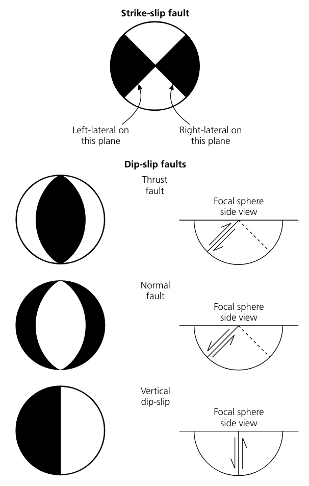
Focal Mechanism Beachball

Radiation pattern

What can we learn from millions of earthquakes?

• Earthquake catalog
• Earthquake statistics
• Earthquake triggering
• Earthquake forecasting
• Fault zone structure
• Seismic tomography
• Volcano, glacier, and landslide monitoring

How is this information used?

• Monitoring earthquakes and earthquake early warning
• Understand earthquake source physics
• Understanding the Earth's structure
• Applying seismology to environmental science, planetary science, climate science, etc.

Detection, learned

Generalized similarity search

Background: Semantic Segmentation vs. Classification

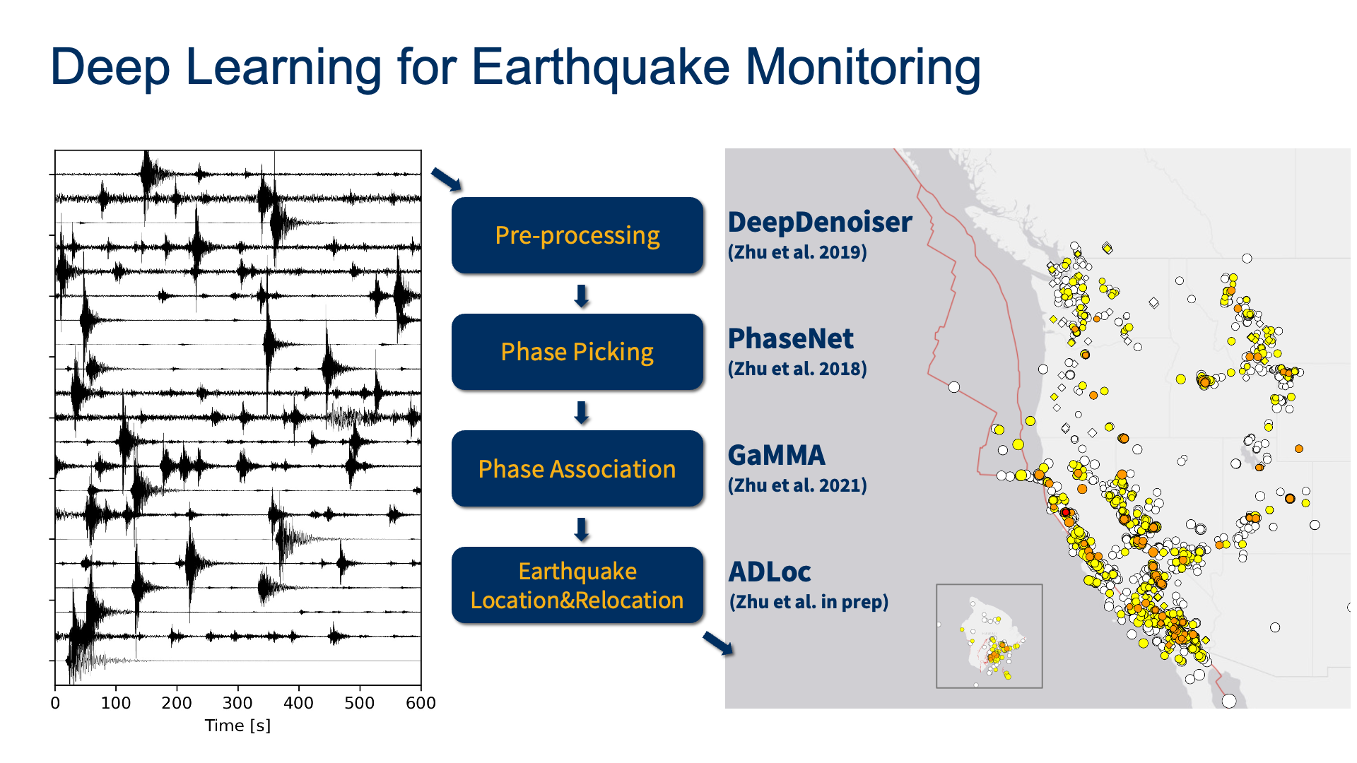
Generalized seismic phase detection with deep learning

PhaseNet

EQTransformer for simultaneous earthquake detection and phase picking

Next-Generation Seismic Monitoring with Neural Operators (PhaseNO)

Clustering-based (Unsupervised), e.g. GaMMA

Clustering

Deep Denoiser

• Short-time Fourier Transform (STFT) + Wiener Filter + Neural Network

Deep learning for earthquake statistics

Large training dataset + Clear objective function

What deep learning costs

• Pros:
  • Robust to noise
  • Sensitive to small earthquakes
  • Fast prediction
• Cons:
  • Need large amount of labeled data
  • Black box
  • Generalization ability

Things to learn in this course

• Familiar with seismic data
• Learn the state-of-the-art machine learning methods for seismic data processing
• Process seismic data, build seismic catalogs, and analyzing seismicity
• Learn basic inverse theory for earthquake location, focal mechanism, seismic tomography, etc.

Schedule

Final project

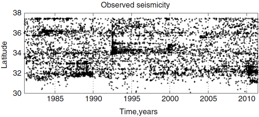
The Geysers - the most seismically active field in California, where the shaking is a side effect of an industrial process.

Grading

• Homework (40%)
• Final project (60%)

Earthquake faults

Earthquakes may be idealized as movement across a planar fault of arbitrary orientation

• strike: , the azimuth of the fault from north where it intersects a horizontal surface
  
• dip: , the angle from the horizontal
  
• rake: , the angle between the slip vector and the strike
  

Earthquake faults

Thrust faulting: reverse faulting on faults with dip angles less than 45
Overthrust faults: Nearly horizontal thrust faults
Strike-slip faulting: horizontal motion between the fault surfaces
Dip-slip faulting: vertical motion
Right-lateral strike–slip motion: standing on one side of a fault, sees the adjacent block move to the right
: left-lateral faulting
: right-lateral faulting
The San Andreas Fault: Right-lateral fault

Earthquake double couple

• An earthquake is usually modeled as slip on a fault, a discontinuity in displacement across an internal surface in the elastic media.
• Internal forces resulting from an explosion or stress release on a fault must act in opposing directions so as to conserve momentum.
• A force couple is a pair of opposing point forces separated by a small distance
• A double couple is a pair of complementary couples that produce no net torque

Moment tensor

We define the force couple as a pair of equal and opposite forces pointing in the direction and separated by a unit distance in the direction.

The magnitude of is the product of the force and the distance .

The condition that angular momentum be conserved requires that is symmetric (e.g., ).

Moment tensor

For example, right-lateral movement on a vertical fault oriented in the direction corresponds to the moment tensor representation

where is the scalar seismic moment:

where is the shear modulus, is the average fault displacement, and is the area of the fault.

The units for are Nm (or dynecm), the same as for force couples.

Global CMT catalog

Global Centroid Moment Tensor

Beach balls

Basic types of faulting

First-motion polarity

Magnitude

The magnitude of the equivalent body forces is
The scalar seismic moment of the earthquake; units of dyn-cm, or N-m

Global earthquakes: body wave magnitude

where A is the ground displacement in microns, T is the dominant period of the measured waves, is the epicentral distance in degrees, and Q is an empirical function of range and event depth h.

• Why ?
• h?

Global earthquakes: surface wave magnitude

For Rayleigh waves on vertical instruments:

Since the strongest Rayleigh wave arrivals are generally at a period of 20 s, this expression is often written as

• Note that this equation is applicable only to shallow events
• surface wave amplitudes are greatly reduced for deep events.

Magnitude saturation

Moment magnitude

The saturation of the and scales for large events helped motivate development of the moment magnitude

where is the moment measured in N-m.

• The advantage of the scale is that it is clearly related to a physical property of the source and it does not saturate for even the largest earthquakes.
• One unit increase in corresponds to a times increase in the moment.
• A earthquake releases about 1000 times more energy than a event.

Magnitude as a function of moment

USGS Magnitude Types; Latest earthquake

The intensity scale

The local strength of ground shaking as determined by damage to structures and the perceptions of people who experienced the earthquake.

• One earthquake can have different intensities at different locations.

USGS Latest Earthquakes

Signal Processing 101

• Fourier Transform (FFT)
• Filtering
• Spectrogram
• Convolution and Cross-correlation
• Short-time Fourier Transform (STFT)
• Wavelet Transform
• Hilbert Transform
• ...

Fourier Transform

Fourier Transform (FT) is a mathematical operation that decomposes a function into its constituent frequencies.

The Fourier Transform of a function is given by:

The inverse Fourier Transform is given by:

Fourier Transform (cont.)

Fourier Transform

Filtering

Filtering is a process of removing unwanted components or features from a signal.

Convolution

Convolution is a mathematical operation on two functions and that produces a third function that expresses how the shape of one is modified by the other.

Cross-correlation

Cross-correlation is a measure of similarity of two series as a function of the displacement of one relative to the other.

Cross-correlation in Frequency Domain

Amplitude threshold

• PGA (Peak Ground Acceleration)
• PGV (Peak Ground Velocity)
• Displacement

Recent M4.5 earthquake

Amplitude threshold

• Pros:
  • Simple and fast
  • Physical parameter
  • Directly related to shaking/damage
• Cons:
  • Limit to large earthquakes
  • Need background noise level for small earthquakes
• Improvements:
  • How to make the threshold adaptive to the background noise level?

STA/LTA

• STA/LTA = Short-Term Average / Long-Term Average

STA/LTA

Template matching / Matched filter

Review of convolution and cross-correlation in last lecture: cross-correlation

Notebook: cross-correlation

(QTM) Quake Template Matching

Template matching / Matched filter

• Pros:
  • Robust to noise
  • More sensitive to small earthquakes
• Cons:
  • High computational cost
  • Need existing catalog to build templates
  • Limited to waveform similarity with templates

FAST (Fingerprint And Similarity Thresholding)

Similarity search

• Pros:
  • Sensitive to small earthquakes
  • Computational efficient
• Cons:
  • Detect all repeating signals
  • Complex to implement

Seismic waves

Seismic phases

Demo: Segment Anything Model (SAM)

Try the SAM model: link

Grid-search / Back-projection, e.g. REAL

Zhang, Ellsworth & Beroza (2019), Rapid Earthquake Association and Location, SRL

Graph-Neural-Network-based, e.g. GENIE

McBrearty & Beroza (2023), Earthquake Phase Association with Graph Neural Networks, BSSA

K-means

Gaussian Mixture Model (GMM)

Gaussian Mixture Model Association (GaMMA)

How to solve an optimization/inversion problem?

• Forward function
• Objective/Loss function
• Gradient
• Optimizer

Locating earthquake using absolute arrival times

notebook

Earthquake location problem:

• Given:
  • Observed arrival times at multiple stations
  • Velocity model
• Goal:
  • Locate the hypocenter and origin time of the earthquake

Forward function:

where is the predicted arrival time at station , is the forward non-linear function (e.g., ray tracing or eikonal equation), and is the model parameter (e.g., source location, origin time, and velocity).

For a uniform velocity:

where is the location of the -th station, is the location of the source, is the origin time, and is the uniform velocity.

Objective/Loss function:

The difference between the observed and predicted times is:

Loss functions:

• Mean squared error (MSE):
• Absolute error:
• Huber loss:

Iterative location methods

where is the initial model, is the perturbation of .

Iterative location methods

We seek to find the that

can be obtained using standard least squares. Next, we set to and repeat the process until the location converges.

How to evaluate the results of earthquake location?

How do we define the "best" location?

The average least square residual:

is called the variance of the residuals, where is the number of degrees of freedom.

A common term is variance reduction (VR), which is defined as:

How to define the uncertainty in the location?

Based on least squares and L2 norm, we define:

where is the uncertainty of the -th residual.

The distribution approximate the degree of freedom of the residuals .

The distribution

The distribution is a probability distribution that describes the sum of the squares of independent standard normal random variables.

The probability density function of the distribution is:

90% confidence interval of

The 90% confidence interval of the distribution is bounded by:

Table for :

How to apply to real data?

Note that the are critical in the analysis, which is based on the assumption that the data misfit are random, uncorrelated, and have a Gaussian distribution.

The estimated data uncertainty is often estimated from the residual of the best location:

where is the best-fitting location.

Then we can use the estimated to calculate the value; then obtain an estimate of the 95% confidence ellipse for the solution.

Challenges: unmodeled velocity heterogeneity

Case: Earthquakes located along a fault will often be mislocated if the seismic velocity changes across the fault.

Challenges: trade-off between event depth and origin time

Case: Earthquake locations for events outside of a network are often not well constrained.

Mitigations:

• time can be used to estimate the source-receiver range at each station
• Adding depth phase (using the differential time ) can help constrain the depth

Locating earthquake using relative arrival times

notebook

In the common situation where the location error is dominated by the biasing effects of unmodeled 3-D velocity structure, the relative location among events within a localized region can be determined with much greater accuracy than the absolute location of any of the events.

HypoDD: Double-difference earthquake location

where and are the observed and predicted arrival times at the -th station for the -th earthquake, respectively.

GrowClust: A Hierarchical Clustering Algorithm for Relative Earthquake Relocation

Review: clustering

More on: Uncertainty

• Aleatoric uncertainty
  • The irreducible part of the uncertainty
  • Uncertainty due to inherent randomness, e.g., the outcome of flipping a coin
• Epistemic uncertainty
  • The reducible part of the uncertainty
  • Uncertainty due to lack of knowledge, e.g., lack of data

Uncertainty Quantification

• Standard deviation of slope and intercept of linear regression
• Bootstrapping
• Markov Chain Monte Carlo (MCMC)
• Hamiltonian Monte Carlo (HMC)
• Stein Variational Gradient Descent (SVGD)
• Dropout as a Bayesian Approximation

HypoSVI: Hypocentre inversion with Stein variational inference

The Earthquake Cycle

Elastic rebound

Spring-block model

When the force exerted by the spring exceeds the static friction , the block will slide until the dynamic friction balances the reduced level of stress.
If , , and are all constant, then the “earthquakes” will repeat at regular recurrence intervals.

Parkfield earthquake

Significant earthquakes at Parkfield, California, have repeated at fairly regular intervals since 1850, leading to predictions of another event before 1993. However the earthquake did not occur until 2004.

Aftershocks

Earthquakes are thought to trigger aftershocks either from the dynamic effects of their radiated seismic waves or the resulting permanent static stress changes

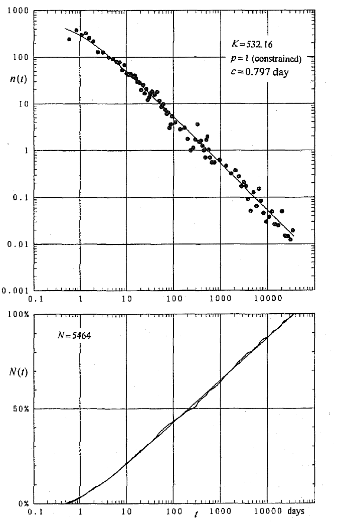
• The seismicity rate decays with time, following a power law relationship, called Omori’s law after Omori (1894)

• Coulomb failure function (CFF)

where is the shear traction on the fault, is the normal traction (positive for tension), is the pore fluid pressure, and is the coefficient of static friction.

Earthquake Source Parameters

• Magnitude
• Origin time
• Location
• Focal mechanism
• Stress drop
• Energy
• Frequency
• ...

Statistical relationship between source parameters

wiki

• Gutenberg-Richter Law (1944)
• Omori Law (1894)
• Båth's Law (1965)
• The Epidemic Type Aftershock Sequence (ETAS) model (1988)
• ...

The Gutenberg-Richter Law

Where:

• is the number of events greater or equal to
• is magnitude
• and are constants

The Gutenberg-Richter Law

The Gutenberg-Richter Law

What controls the slope ?

Temporal variation of

The magnitude completeness ()

What affects the magnitude completeness?

• Station coverage
• Background noise
• Detection algorithms
• ...

Omori Law

The number of events in time after the mainshock

A modified Omori Law

𝐾: productivity of aftershocks
𝑝: decay rate
c: delay time

The decay rate

• valid for a long time range
• independent of magnitude

The aftershock productivity

• Combined with the Gutenberg-Richter law

The Epidemic Type Aftershock Sequence (ETAS) model

The Epidemic Type Aftershock Sequence (ETAS) model

• is the background rate
• is the productivity
• is the magnitude completeness
• is the decay rate
• is the delay time
• is the magnitude scaling
• is the occurrence times of previous earthquakes.

The ETAS model

• Modeling earthquake activity of a Poissonian background and a cluster process
• Analyzing “background” or “clustered” events
• Most widely used model for earthquake forecasting

Coulomb failure stress (CFS) (Static triggering)

: change in shear stress
: change in normal stress (positive for tension)
: change in pore pressure
: friction coefficient

Earthquake swarms

“[a sequence] where the number and the magnitude of earthquakes gradually increase with time, and then decreases after a certain period. There is no single predominant principal earthquake” - Mogi (1963)

How to determine focal mechanism?

Review: Inverse Problems in Geophysics

• Forward function: last lecture
• Objective/Loss function
• Gradient
• Optimizer

Focal mechanism from first motion polarity

• FPFIT

Objective/Loss function:

and are the observed and theoretical first-motion polarity (0.5 for compression, -0.5 for dilatation).
is the square root of the normalized theoretical P-wave radiation amplitude of earthquake recorded at the station for source model .