Previous slide Next slide Toggle fullscreen Open presenter view
The Earthquake Cycle
Spring-block model
When the force exerted by the spring exceeds the static friction
Earthquake recurrence model
Parkfield earthquake
Significant earthquakes at Parkfield, California, have repeated at fairly regular intervals since 1850, leading to predictions of another event before 1993. However the earthquake did not occur until 2004.
The block-slider model
A problem with the characteristic earthquake hypothesis is that it ignores the interactions with adjacent segments on the same fault, as well as interactions with other faults
Self-similar and fractial scaling relationship
Power-law distribution of seismicity rates (the b-value relationship)
Nearly constant value of stress drop over a wide range of earthquake sizes
Fractal dimension D approximately twice the b-value (Turcotte, 1997)
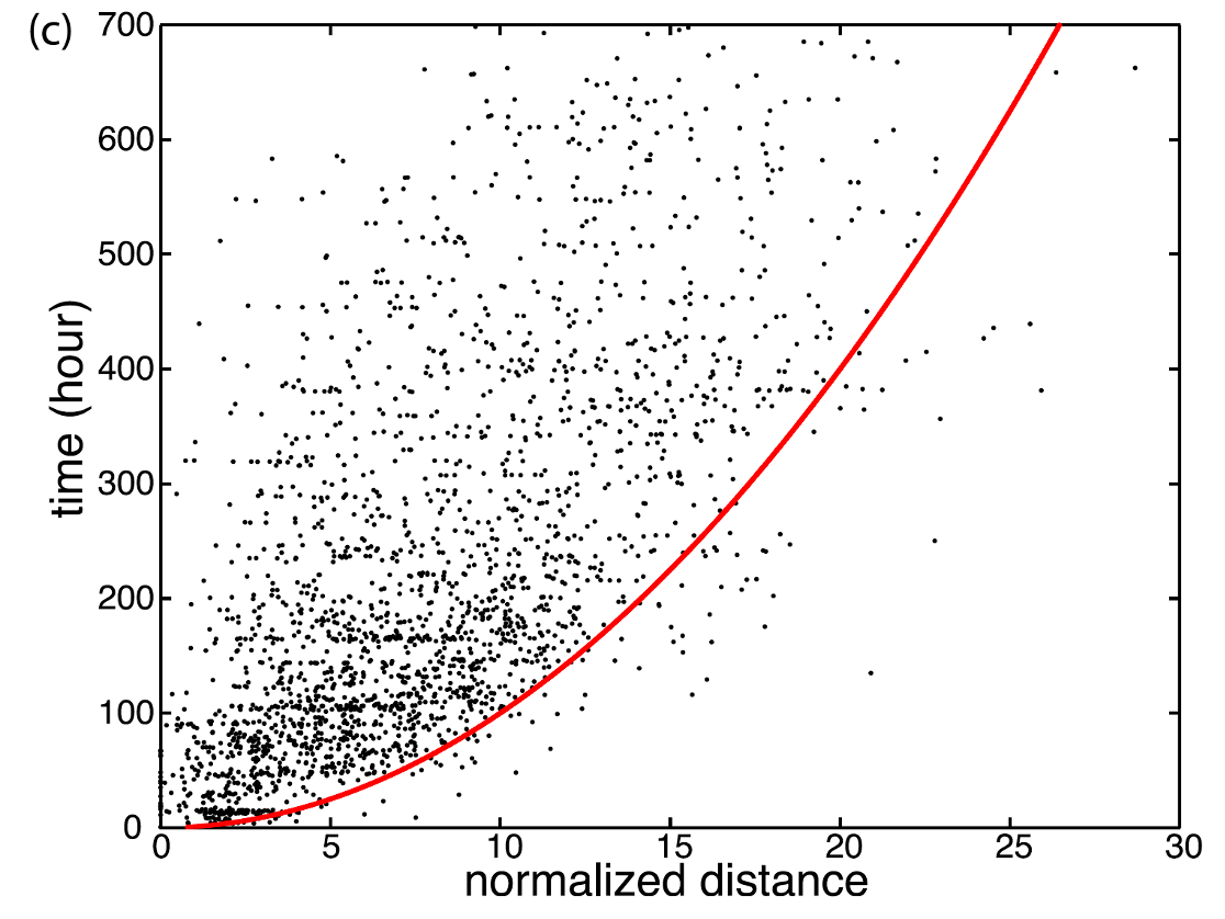
Aftershocks
Earthquakes are thought to trigger aftershocks either from the dynamic effects of their radiated seismic waves or the resulting permanent static stress changes
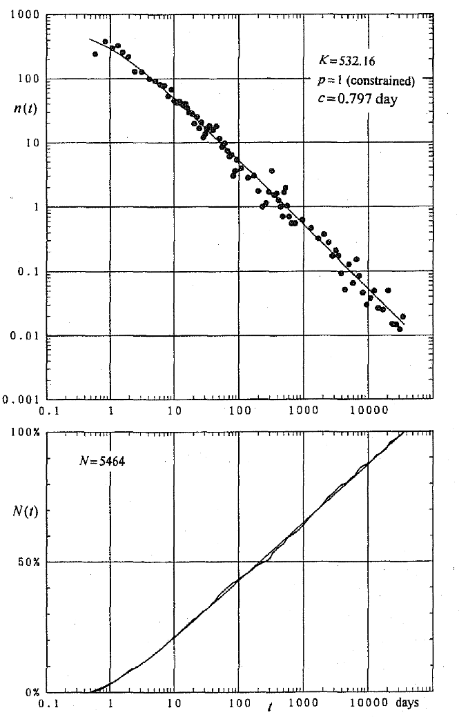
The seismicity rate decays with time, following a power law relationship, called Omori’s law after Omori (1894)
Coulomb failure function (CFF)
where
Earthquake Source Parameters
Magnitude
Origin time
Location
Focal mechanism
Stress drop
Energy
Frequency
...
Statistical relationship between source parameters
wiki
Gutenberg-Richter Law (1944)
Omori Law (1894)
Båth's Law (1965)
The Epidemic Type Aftershock Sequence (ETAS) model (1988)
...
The Gutenberg-Richter Law
Where:
The Gutenberg-Richter Law
The Gutenberg-Richter Law
What controls the slop
Temporal variation of
Temporal variation of
The magnitude completeness (
What affects the magnitude completeness?
Station coverage
Background noise
Detection algorithms
...
Omori Law
The number of events
A modified Omori Law
𝐾: productivity of aftershocks
The decay rate
valid for a long time range
independent of magnitude
The aftershock productivity
Combined with the Gutenberg-Richter law
(Reasenberg and Jones 1989)
How about for foreshocks?
The Epidemic Type Aftershock Sequence (ETAS) model
The Epidemic Type Aftershock Sequence (ETAS) model
The ETAS model
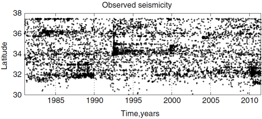
Modeling earthquake activity of a Poissonian background and a cluster process
Analyzing “background” or “clustered” events
Most widely used model for earthquake forecasting
Incorporate spatial triggering into ETAS
Physical models on aftershocks spatial distribution
Coulomb failure stress (CFS) (Static triggering)
(Stein and Lisowski 1983)
Coulomb failure stress (CFS)
Dynamic triggering
Dynamic triggering
Earthquake swarms
“[a sequence] where the number and the magnitude of earthquakes gradually increase with time, and then decreases after a certain period. There is no single predominant principal earthquake” - Mogi (1963)
2012 Brawley,CA swarm
2018 Pahala,Hawaii swarm
2018 Pahala,Hawaii swarm
Spatial-temporal evolution patterns of swarms
Deep learning for earthquake statistics
Deep learning of aftershock patterns following large earthquakes, Devries et al. 2018
Deep learning for earthquake statistics
Using Deep Learning for Flexible and Scalable Earthquake Forecasting, Kelian et al. 2023
Deep learning for earthquake statistics
Using Deep Learning for Flexible and Scalable Earthquake Forecasting, Kelian et al. 2023
Deep learning for earthquake statistics
A neural encoder for earthquake rate forecasting, Zlydenko et al. 2023
Class project datasets:
- [Nodal Seismic Experiment at the Berkeley Section of the Hayward Fault](https://pubs.geoscienceworld.org/ssa/srl/article/93/4/2377/613344/Nodal-Seismic-Experiment-at-the-Berkeley-Section) (Taka'aki et al. 2022)
- An island on Mid-Atlantic Ridge: [Networks](http://ds.iris.edu/gmap/#maxlat=73.3732&maxlon=-1.582&minlat=68.7841&minlon=-15.1596&network=*&drawingmode=box&planet=earth), [Seismicity](https://nnsn.geo.uib.no/nnsn/#/)
- [California](https://earthquake.usgs.gov/earthquakes/map/?extent=30.25907,-128.67188&extent=42.65012,-109.51172&range=month&magnitude=all&listOnlyShown=true&settings=true)
---
### Clustering analysis of earthquakes

**Aggregating 18 swarms in southen California**