Neural Networks 1

Regression and Classification with Neural Networks¶

Run in Google Colab

Created by Minh-Chien Trinh, Jeonbuk National University,

1.1. A Brief History¶

In the 1940s, NNs were conceived.

In the 1960s, the concept of backpropagation came, then people know how to train them.

In 2010, NNs started winning competitions and get much attention than before.

Since 2010, NNs have been on a meteoric rise as their magical ability to solve problems previously deemed unsolvable (i.e., image captioning, language translation, audio and video synthesis, and more).

One important milestone is the AlexNet architecture in 2012, which won the ImageNet competition.

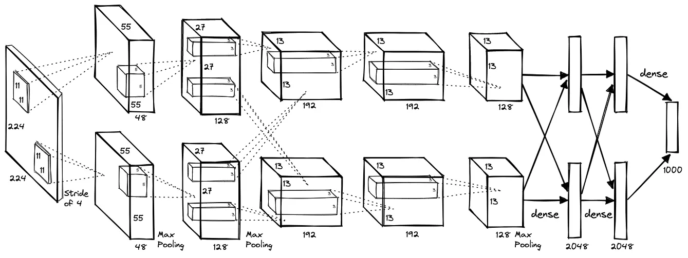
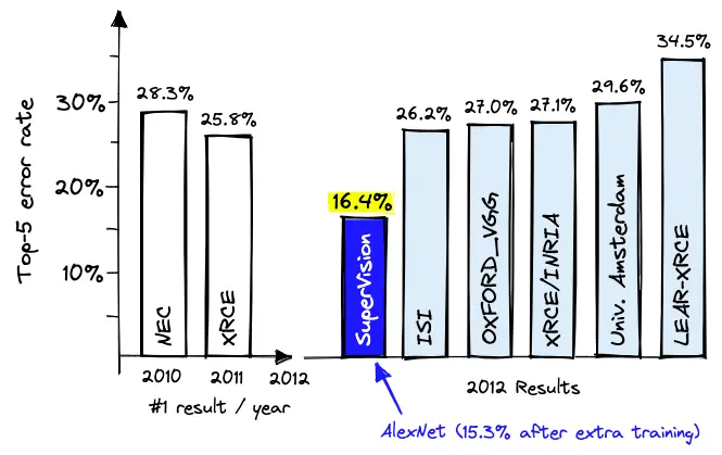
The ImageNet competition is a benchmark for image classification, where the goal is to classify images into one of 1,000 categories.

You can find more information about the AlexNet model on Wikipedia. We will use the AlexNet model in the next lecture to classify images of rocks.

Currently, NNs are the primary solution to most competitions and technological challenges like self-driving cars, calculating risk, detecting fraud, early cancer detection,…

1.2. What is a Neural Network?¶

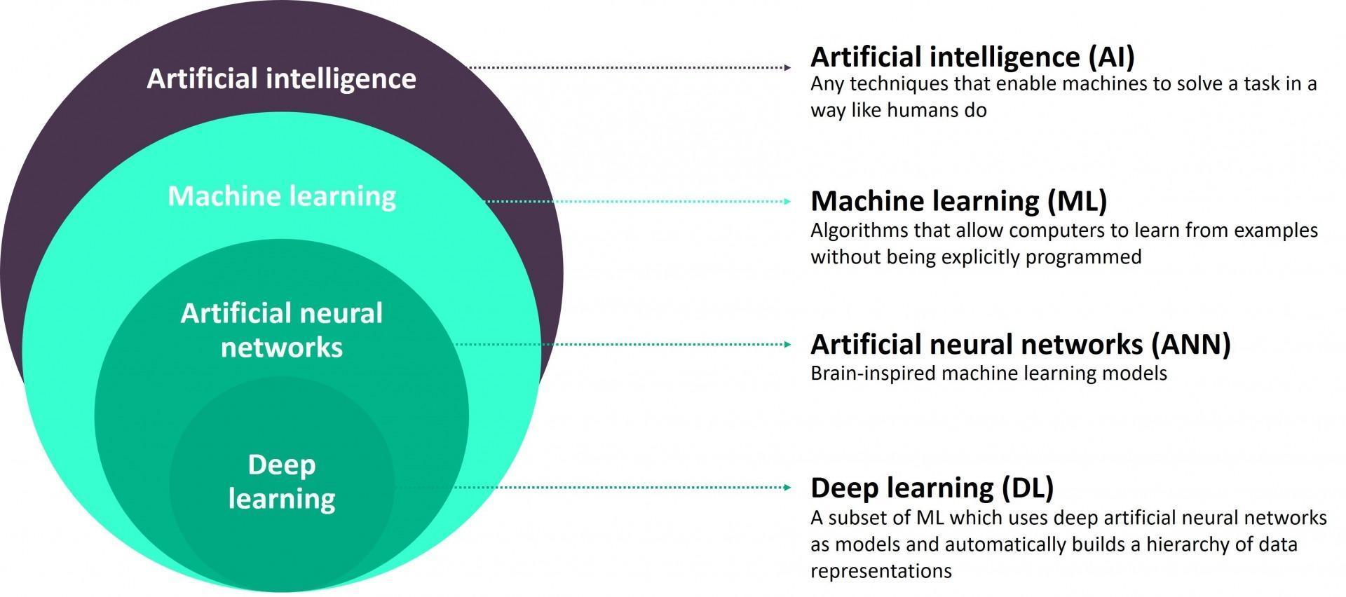
ANNs are inspired by the organic brain, translated to the computer.

ANNs have neurons, activations, and interconnectivities.

NNs are considered “black boxes” between inputs and outputs.

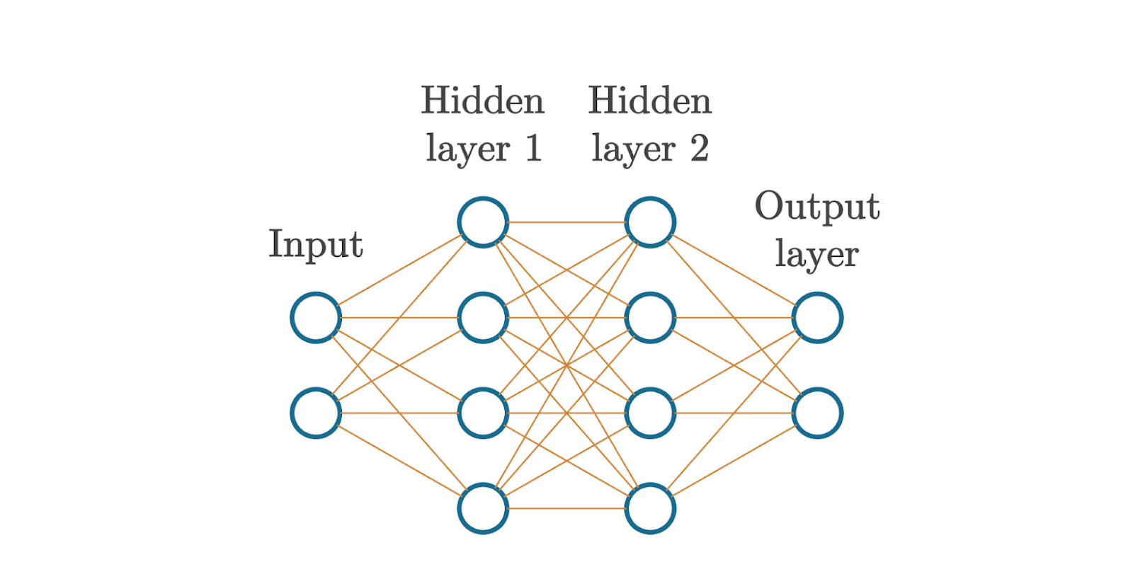
Each connection between neurons has a weight associated with it. Weights are multiplied by corresponding input values. These multiplications flow into the neuron and are summed before being added with a bias. Weights and biases are trainable or tunable.

$$ \begin{aligned} output & = weight \cdot input + bias \\ y & = a \cdot x + b \end{aligned} $$

The formula should look very familiar to you. It is similar to the previous linear regression and classification models.

Then, an activation function is applied to the output.

$$ \begin{aligned} output & = \sum (weight \cdot input) + bias \\ output & = activation (output) \end{aligned} $$

When a step function that mimics a neuron in the brain (i.e., “firing” or not, on-off switch) is used as an activation function:

• If its output is greater than 0, the neuron fires (it would output 1).
• If its output is less than 0, the neuron does not fire and would pass along a 0.

The input layer represents the actual input data (i.e., pixel values from an image, temperature, …)

• The data can be “raw”, should be preprocessed like normalization and scaling.
• The input needs to be in numeric form.

The output layer is whatever the NN returns.

• In regression, the predicted value is a scalar value, the output layer has a single neuron.
• In classification, the class of the input is predicted, the output layer has as many neurons as the training dataset has classes. But can also have a single output neuron for binary (two classes) classification.

A typical NN has thousands or even up to millions of adjustable parameters (weights and biases).

NNs act as enormous functions with vast numbers of parameters.

Finding the combination of parameter (weight and bias) values is the challenging part.

The end goal for NNs is to adjust their weights and biases (the parameters), so they produce the desired output for unseen data.

A major issue in supervised learning is overfitting, where the algorithm doesn’t understand underlying input-output dependencies, just basically “memorizes” the training data.

The goal of NN is generalization, that can be obtained when separating the data into training data and validation data.

Weights and biases are adjusted based on the error/loss presenting how “wrong” the algorithm in NN predicting the output.

NNs can be used for regression (predict a scalar, singular, value), clustering (assigned unstructured data into groups), and many other tasks.

If you want to learn more about Deep Learning (Deep Nerual Networks), you can check the Deep Learning Specialization on Coursera or watch videos on YouTube.

In this lecture, we will use PyTorch to build and train neural networks. The pytorch library is a powerful tool for building and training neural networks. It provides a flexible and efficient library for deep learning. It is also currently the most popular library for deep learning.

Let's import the necessary libraries of PyTorch and other libraries.

In [1]:

## First part of this semester
import matplotlib.pyplot as plt
import numpy as np
import pandas as pd

## Second part of this semester
from sklearn.impute import SimpleImputer
from sklearn.metrics import r2_score, accuracy_score, confusion_matrix, ConfusionMatrixDisplay
from sklearn.model_selection import train_test_split
from sklearn.preprocessing import LabelEncoder

## Last part of this semester
import torch
import torch.nn as nn
import torch.nn.functional as F
import torch.optim as optim

## First part of this semester import matplotlib.pyplot as plt import numpy as np import pandas as pd ## Second part of this semester from sklearn.impute import SimpleImputer from sklearn.metrics import r2_score, accuracy_score, confusion_matrix, ConfusionMatrixDisplay from sklearn.model_selection import train_test_split from sklearn.preprocessing import LabelEncoder ## Last part of this semester import torch import torch.nn as nn import torch.nn.functional as F import torch.optim as optim

Matplotlib is building the font cache; this may take a moment.

In [2]:

## Set random seed
torch.manual_seed(0)
torch.cuda.manual_seed(0)
np.random.seed(0)

## Set random seed torch.manual_seed(0) torch.cuda.manual_seed(0) np.random.seed(0)

Applying Neural Networks for Regression¶

In today's lecture, we will revisit the Betoule data and apply neural networks for regression.

If you already forgot the background of this data, please review the lecture 04 regression.

Remember the challenge of the Betoule data is that the velocity is non-linear with respect to the distance.

In the previous lecture, we used sklearn to fit the linear regression model with high polynomial degrees.

Here we will use PyTorch to fit the Betoule data and compare the results with the linear regression model.

• Load the Betoule data

In [3]:

## Load the Betoule data
# betoule_data = pd.read_csv('data/mu_z.csv',header=1) ## reading from local file
betoule_data = pd.read_csv('https://raw.githubusercontent.com/AI4EPS/EPS88_PyEarth/refs/heads/main/docs/scripts/data/mu_z.csv',header=1) ## reading from github for running on colab
betoule_data.head()

## Apply processing to convert to distance and velocity
# speed of light in km/s
c = 2.9979e8 / 1000 

# the formula for v from z (and c)
betoule_data['velocity'] = c * (((betoule_data['z']+1.)**2-1.)/((betoule_data['z']+1.)**2+1.)) 

# convert mu to Gpc
betoule_data['distance'] = 10000*(10.**((betoule_data['mu'])/5.))*1e-9

## Load the Betoule data # betoule_data = pd.read_csv('data/mu_z.csv',header=1) ## reading from local file betoule_data = pd.read_csv('https://raw.githubusercontent.com/AI4EPS/EPS88_PyEarth/refs/heads/main/docs/scripts/data/mu_z.csv',header=1) ## reading from github for running on colab betoule_data.head() ## Apply processing to convert to distance and velocity # speed of light in km/s c = 2.9979e8 / 1000 # the formula for v from z (and c) betoule_data['velocity'] = c * (((betoule_data['z']+1.)**2-1.)/((betoule_data['z']+1.)**2+1.)) # convert mu to Gpc betoule_data['distance'] = 10000*(10.**((betoule_data['mu'])/5.))*1e-9

In [4]:

## Review the data
plt.figure()
plt.scatter(betoule_data['distance'],betoule_data['velocity'])
plt.xlabel('Distance (Mpc)')
plt.ylabel('Velocity (km s$^{-1}$)')
plt.show()

## Review the data plt.figure() plt.scatter(betoule_data['distance'],betoule_data['velocity']) plt.xlabel('Distance (Mpc)') plt.ylabel('Velocity (km s$^{-1}$)') plt.show()

• Prepare the data into features (X) and target (y). This is same as the previous lecture.

In [5]:

## Define features (X) and target (y)
X = betoule_data[['distance']].values
y = betoule_data[['velocity']].values

## Split the data into training and test sets using 30% of the data for testing
X_train, X_test, y_train, y_test = train_test_split(X, y, test_size=0.3, random_state=41)

## Define features (X) and target (y) X = betoule_data[['distance']].values y = betoule_data[['velocity']].values ## Split the data into training and test sets using 30% of the data for testing X_train, X_test, y_train, y_test = train_test_split(X, y, test_size=0.3, random_state=41)

• Let's start to build the first neural network model to fit the Betoule data.

In [6]:

## Convert data to PyTorch tensors
X_train_tensor = torch.tensor(X_train, dtype=torch.float32)
y_train_tensor = torch.tensor(y_train, dtype=torch.float32)
X_test_tensor = torch.tensor(X_test, dtype=torch.float32)
y_test_tensor = torch.tensor(y_test, dtype=torch.float32)

## Normalize the data to make the training process more efficient
magnitude_X = 10**int(np.log10(X.max()))
magnitude_y = 10**int(np.log10(y.max()))
X_train_tensor = X_train_tensor / magnitude_X
y_train_tensor = y_train_tensor / magnitude_y
X_test_tensor = X_test_tensor / magnitude_X
y_test_tensor = y_test_tensor / magnitude_y

## Define the neural network model
class SimpleNN(nn.Module):
    def __init__(self, input_size, output_size, hidden_size):
        super(SimpleNN, self).__init__()
        ## Define the neural network layers
        self.fc1 = nn.Linear(input_size, hidden_size)
        self.fc2 = nn.Linear(hidden_size, output_size)  
    
    def forward(self, x):
        ## Apply the neural network layers
        x = self.fc1(x)
        x = F.relu(x)
        x = self.fc2(x)
        return x

## Initialize the model, loss function, and optimizer
input_size = X.shape[-1]
output_size = 1 # Output layer for regression (1 output neuron)
hidden_size = 16

model = SimpleNN(input_size, output_size, hidden_size)
criterion = nn.MSELoss()
optimizer = optim.Adam(model.parameters(), lr=0.1)

## Define fit function
def fit(model, X, y, epochs=100):
    model.train()
    losses = []
    for epoch in range(epochs):
        optimizer.zero_grad()
        outputs = model(X)
        loss = criterion(outputs, y)
        loss.backward()
        optimizer.step()
        losses.append(loss.item())
        if (epoch+1) % 10 == 0:
            print(f'Epoch [{epoch+1}/{epochs}], Loss: {loss.item():.4f}')
    return losses

## Define predict function
def predict(model, X):
    model.eval()
    with torch.no_grad():
        outputs = model(X)
    return outputs

## Train the model
losses = fit(model, X_train_tensor, y_train_tensor, epochs=100)

## Plot the loss during the training process
plt.figure()
plt.plot(losses)
plt.xlabel('Epochs')
plt.ylabel('Loss')
plt.show()

## Convert data to PyTorch tensors X_train_tensor = torch.tensor(X_train, dtype=torch.float32) y_train_tensor = torch.tensor(y_train, dtype=torch.float32) X_test_tensor = torch.tensor(X_test, dtype=torch.float32) y_test_tensor = torch.tensor(y_test, dtype=torch.float32) ## Normalize the data to make the training process more efficient magnitude_X = 10**int(np.log10(X.max())) magnitude_y = 10**int(np.log10(y.max())) X_train_tensor = X_train_tensor / magnitude_X y_train_tensor = y_train_tensor / magnitude_y X_test_tensor = X_test_tensor / magnitude_X y_test_tensor = y_test_tensor / magnitude_y ## Define the neural network model class SimpleNN(nn.Module): def __init__(self, input_size, output_size, hidden_size): super(SimpleNN, self).__init__() ## Define the neural network layers self.fc1 = nn.Linear(input_size, hidden_size) self.fc2 = nn.Linear(hidden_size, output_size) def forward(self, x): ## Apply the neural network layers x = self.fc1(x) x = F.relu(x) x = self.fc2(x) return x ## Initialize the model, loss function, and optimizer input_size = X.shape[-1] output_size = 1 # Output layer for regression (1 output neuron) hidden_size = 16 model = SimpleNN(input_size, output_size, hidden_size) criterion = nn.MSELoss() optimizer = optim.Adam(model.parameters(), lr=0.1) ## Define fit function def fit(model, X, y, epochs=100): model.train() losses = [] for epoch in range(epochs): optimizer.zero_grad() outputs = model(X) loss = criterion(outputs, y) loss.backward() optimizer.step() losses.append(loss.item()) if (epoch+1) % 10 == 0: print(f'Epoch [{epoch+1}/{epochs}], Loss: {loss.item():.4f}') return losses ## Define predict function def predict(model, X): model.eval() with torch.no_grad(): outputs = model(X) return outputs ## Train the model losses = fit(model, X_train_tensor, y_train_tensor, epochs=100) ## Plot the loss during the training process plt.figure() plt.plot(losses) plt.xlabel('Epochs') plt.ylabel('Loss') plt.show()

Epoch [10/100], Loss: 0.0607
Epoch [20/100], Loss: 0.0178
Epoch [30/100], Loss: 0.0206
Epoch [40/100], Loss: 0.0087
Epoch [50/100], Loss: 0.0040
Epoch [60/100], Loss: 0.0028
Epoch [70/100], Loss: 0.0019
Epoch [80/100], Loss: 0.0012
Epoch [90/100], Loss: 0.0009
Epoch [100/100], Loss: 0.0007

• Evaluate the model on the test set. This is same as the previous lecture.

In [7]:

## Predict on the test set
y_pred_tensor = predict(model, X_test_tensor)
y_pred = y_pred_tensor.numpy() * magnitude_y

## Calculate R-squared metric
r2 = r2_score(y_test, y_pred)
print(f'R-squared: {r2:.4f}')

## Predict on the test set y_pred_tensor = predict(model, X_test_tensor) y_pred = y_pred_tensor.numpy() * magnitude_y ## Calculate R-squared metric r2 = r2_score(y_test, y_pred) print(f'R-squared: {r2:.4f}')

R-squared: 0.9950

In [8]:

## Plot the results

## Predict on the whole dataset for plotting
X_tensor = torch.tensor(X, dtype=torch.float32)
X_tensor = X_tensor / magnitude_X
y_pred_tensor = predict(model, X_tensor)
y_pred = y_pred_tensor.numpy() * magnitude_y
y_pred = y_pred.squeeze() # remove the extra dimension

plt.figure(figsize=(6, 6))
plt.subplot(2,1,1)
plt.scatter(betoule_data['distance'],betoule_data['velocity'])
plt.plot(betoule_data['distance'],y_pred,color='orange',)
plt.title('data and a nerual network fit')
plt.ylabel('Velocity (km s$^{-1}$)')
plt.xlabel('Distance (Mpc)')

plt.subplot(2,1,2)
plt.scatter(betoule_data['distance'],betoule_data['velocity']-y_pred)
plt.title('residuals of nerual network fit')
plt.ylabel('Residual velocity (km s$^{-1}$)')
plt.xlabel('Distance (Mpc)')

plt.tight_layout()
plt.show()

## Plot the results ## Predict on the whole dataset for plotting X_tensor = torch.tensor(X, dtype=torch.float32) X_tensor = X_tensor / magnitude_X y_pred_tensor = predict(model, X_tensor) y_pred = y_pred_tensor.numpy() * magnitude_y y_pred = y_pred.squeeze() # remove the extra dimension plt.figure(figsize=(6, 6)) plt.subplot(2,1,1) plt.scatter(betoule_data['distance'],betoule_data['velocity']) plt.plot(betoule_data['distance'],y_pred,color='orange',) plt.title('data and a nerual network fit') plt.ylabel('Velocity (km s$^{-1}$)') plt.xlabel('Distance (Mpc)') plt.subplot(2,1,2) plt.scatter(betoule_data['distance'],betoule_data['velocity']-y_pred) plt.title('residuals of nerual network fit') plt.ylabel('Residual velocity (km s$^{-1}$)') plt.xlabel('Distance (Mpc)') plt.tight_layout() plt.show()

• Compare the results with previous polynomial regression. How does the neural network perform?

Applying Neural Networks for Classification¶

Neural networks work well for the regression tasks, how about the classification tasks?

Let's continue to apply neural networks for the binary classification task.

Again, we will re-use the basalt affinity dataset that we covered in the previous lecture.

If you already forgot the background of this data, please review the lecture 05 classification.

• Load the basalt affinity data

In [9]:

## Load the basalt affinity data
# basalt_data = pd.read_csv('data/Vermeesch2006.csv')
basalt_data = pd.read_csv('https://raw.githubusercontent.com/AI4EPS/EPS88_PyEarth/refs/heads/main/docs/scripts/data/Vermeesch2006.csv') # for running on colab
basalt_data.tail()

## Load the basalt affinity data # basalt_data = pd.read_csv('data/Vermeesch2006.csv') basalt_data = pd.read_csv('https://raw.githubusercontent.com/AI4EPS/EPS88_PyEarth/refs/heads/main/docs/scripts/data/Vermeesch2006.csv') # for running on colab basalt_data.tail()

Out[9]:

	affinity	SiO2_wt_percent	TiO2_wt_percent	Al2O3_wt_percent	Fe2O3_wt_percent	FeO_wt_percent	CaO_wt_percent	MgO_wt_percent	MnO_wt_percent	K2O_wt_percent	...	Hf_ppm	Ta_ppm	Pb_ppm	Th_ppm	U_ppm	143Nd/144Nd	87Sr/86Sr	206Pb/204Pb	207Pb/204Pb	208Pb/204Pb
751	IAB	50.97	0.78	18.86	NaN	NaN	10.85	4.71	0.16	0.60	...	NaN	NaN	NaN	NaN	NaN	NaN	NaN	18.82	15.556	38.389
752	IAB	51.00	1.41	17.06	3.80	7.04	9.97	4.96	0.17	0.73	...	NaN	NaN	NaN	NaN	NaN	NaN	0.70348	NaN	NaN	NaN
753	IAB	52.56	1.21	17.74	2.28	7.53	10.48	5.57	0.24	0.29	...	NaN	NaN	NaN	NaN	NaN	NaN	0.70362	NaN	NaN	NaN
754	IAB	52.59	1.50	16.88	2.41	7.90	10.83	4.91	0.26	0.54	...	NaN	NaN	NaN	NaN	NaN	NaN	0.70363	NaN	NaN	NaN
755	IAB	52.96	1.27	15.65	2.91	9.32	9.78	4.24	0.23	0.46	...	NaN	NaN	NaN	NaN	NaN	NaN	0.70352	NaN	NaN	NaN

5 rows × 52 columns

In [10]:

## Review the data
plt.figure(figsize=(8, 6))

for affinity in basalt_data['affinity'].unique():
    subset = basalt_data[basalt_data['affinity'] == affinity]
    plt.scatter(subset['TiO2_wt_percent'], subset['V_ppm'], label=affinity, edgecolor='k', s=50)

plt.legend()
plt.xlabel('TiO2 (wt%)')
plt.ylabel('V (ppm)')
plt.show()

## Review the data plt.figure(figsize=(8, 6)) for affinity in basalt_data['affinity'].unique(): subset = basalt_data[basalt_data['affinity'] == affinity] plt.scatter(subset['TiO2_wt_percent'], subset['V_ppm'], label=affinity, edgecolor='k', s=50) plt.legend() plt.xlabel('TiO2 (wt%)') plt.ylabel('V (ppm)') plt.show()

• Prepare the data into features (X) and target (y). This is same as the previous lecture.

In [11]:

## Prepare the data into features (X) and target (y)
X = basalt_data.drop('affinity', axis=1)
y = basalt_data['affinity']

## Encode the target variable
le = LabelEncoder()
le.fit(y)
y = le.transform(y)

## Impute missing values using median imputation
imputer = SimpleImputer(strategy='median')
X = imputer.fit_transform(X)

## Split the data into training and test sets using 30% of the data for testing
X_train, X_test, y_train, y_test = train_test_split(X, y, test_size=0.3, random_state=41)

## Prepare the data into features (X) and target (y) X = basalt_data.drop('affinity', axis=1) y = basalt_data['affinity'] ## Encode the target variable le = LabelEncoder() le.fit(y) y = le.transform(y) ## Impute missing values using median imputation imputer = SimpleImputer(strategy='median') X = imputer.fit_transform(X) ## Split the data into training and test sets using 30% of the data for testing X_train, X_test, y_train, y_test = train_test_split(X, y, test_size=0.3, random_state=41)

In [12]:

X_train_tensor.shape

X_train_tensor.shape

Out[12]:

torch.Size([21, 1])

• Let's start to build the second neural network model to fit the basalt affinity data.

In [13]:

## Convert data to PyTorch tensors
X_train_tensor = torch.tensor(X_train, dtype=torch.float32)
y_train_tensor = torch.tensor(y_train, dtype=torch.long)
X_test_tensor = torch.tensor(X_test, dtype=torch.float32)
y_test_tensor = torch.tensor(y_test, dtype=torch.long)

## Normalize the data to make the training process more efficient
mu = X_train_tensor.mean(dim=0, keepdim=True)
std = X_train_tensor.std(dim=0, keepdim=True)
X_train_tensor = (X_train_tensor - mu) / std
X_test_tensor = (X_test_tensor - mu) / std

## Define the neural network model
class SimpleNN(nn.Module):
    def __init__(self, input_size,  output_size, hidden_size):
        super(SimpleNN, self).__init__()
        ## Define the neural network layers
        self.fc1 = nn.Linear(input_size, hidden_size)
        self.fc2 = nn.Linear(hidden_size, output_size)
    
    def forward(self, x):
        ## Apply the neural network layers
        x = self.fc1(x)
        x = F.relu(x)
        x = self.fc2(x)
        return x

## Initialize the model, loss function, and optimizer
input_size = X_train.shape[-1]
output_size = len(le.classes_) # Output layer for classification (number of classes)
hidden_size = 16

model = SimpleNN(input_size, output_size, hidden_size)
criterion = nn.CrossEntropyLoss()
optimizer = optim.Adam(model.parameters(), lr=0.1)

## Define fit function
def fit(model, X_train, y_train, epochs=100):
    model.train()
    losses = []
    for epoch in range(epochs):
        optimizer.zero_grad()
        outputs = model(X_train)
        loss = criterion(outputs, y_train)
        loss.backward()
        optimizer.step()
        losses.append(loss.item())
        if (epoch+1) % 10 == 0:
            print(f'Epoch [{epoch+1}/{epochs}], Loss: {loss.item():.4f}')
    return losses

## Define predict function
def predict(model, X):
    model.eval()
    with torch.no_grad():
        outputs = model(X)
        _, predicted = torch.max(outputs, 1)
    return predicted

## Train the model
losses = fit(model, X_train_tensor, y_train_tensor, epochs=100)

## Plot the loss
plt.figure()
plt.plot(losses)
plt.xlabel('Epochs')
plt.ylabel('Loss')
plt.show()

## Convert data to PyTorch tensors X_train_tensor = torch.tensor(X_train, dtype=torch.float32) y_train_tensor = torch.tensor(y_train, dtype=torch.long) X_test_tensor = torch.tensor(X_test, dtype=torch.float32) y_test_tensor = torch.tensor(y_test, dtype=torch.long) ## Normalize the data to make the training process more efficient mu = X_train_tensor.mean(dim=0, keepdim=True) std = X_train_tensor.std(dim=0, keepdim=True) X_train_tensor = (X_train_tensor - mu) / std X_test_tensor = (X_test_tensor - mu) / std ## Define the neural network model class SimpleNN(nn.Module): def __init__(self, input_size, output_size, hidden_size): super(SimpleNN, self).__init__() ## Define the neural network layers self.fc1 = nn.Linear(input_size, hidden_size) self.fc2 = nn.Linear(hidden_size, output_size) def forward(self, x): ## Apply the neural network layers x = self.fc1(x) x = F.relu(x) x = self.fc2(x) return x ## Initialize the model, loss function, and optimizer input_size = X_train.shape[-1] output_size = len(le.classes_) # Output layer for classification (number of classes) hidden_size = 16 model = SimpleNN(input_size, output_size, hidden_size) criterion = nn.CrossEntropyLoss() optimizer = optim.Adam(model.parameters(), lr=0.1) ## Define fit function def fit(model, X_train, y_train, epochs=100): model.train() losses = [] for epoch in range(epochs): optimizer.zero_grad() outputs = model(X_train) loss = criterion(outputs, y_train) loss.backward() optimizer.step() losses.append(loss.item()) if (epoch+1) % 10 == 0: print(f'Epoch [{epoch+1}/{epochs}], Loss: {loss.item():.4f}') return losses ## Define predict function def predict(model, X): model.eval() with torch.no_grad(): outputs = model(X) _, predicted = torch.max(outputs, 1) return predicted ## Train the model losses = fit(model, X_train_tensor, y_train_tensor, epochs=100) ## Plot the loss plt.figure() plt.plot(losses) plt.xlabel('Epochs') plt.ylabel('Loss') plt.show()

Epoch [10/100], Loss: 0.1224
Epoch [20/100], Loss: 0.0299
Epoch [30/100], Loss: 0.0067
Epoch [40/100], Loss: 0.0016
Epoch [50/100], Loss: 0.0008
Epoch [60/100], Loss: 0.0005
Epoch [70/100], Loss: 0.0003
Epoch [80/100], Loss: 0.0003
Epoch [90/100], Loss: 0.0002
Epoch [100/100], Loss: 0.0002

• Evaluate the model on the test set. This is same as the previous lecture.

In [14]:

## Predict on the test set
y_pred_tensor = predict(model, X_test_tensor)
y_pred = y_pred_tensor.numpy()

## Calculate accuracy
accuracy = accuracy_score(y_test, y_pred)
print(f'Accuracy: {accuracy:.4f}')

## Confusion matrix
conf_matrix = confusion_matrix(y_test, y_pred)
disp = ConfusionMatrixDisplay(confusion_matrix=conf_matrix, display_labels=le.classes_)
disp.plot(cmap=plt.cm.Blues, values_format='d', colorbar=False);

## Predict on the test set y_pred_tensor = predict(model, X_test_tensor) y_pred = y_pred_tensor.numpy() ## Calculate accuracy accuracy = accuracy_score(y_test, y_pred) print(f'Accuracy: {accuracy:.4f}') ## Confusion matrix conf_matrix = confusion_matrix(y_test, y_pred) disp = ConfusionMatrixDisplay(confusion_matrix=conf_matrix, display_labels=le.classes_) disp.plot(cmap=plt.cm.Blues, values_format='d', colorbar=False);

Accuracy: 0.9075

• Compare the results with previous classification methods. How does the neural network perform?

• Compare the two neural networks built for the regression and classification tasks. Please list the similarities and differences.

• The neural networks we built are very simple with only one hidden layer. Do you know which variable controls the complexity of the neural networks?

• If we want to build a more complex neural network, how can we do it? Think about the number of layers and neurons in each layer.

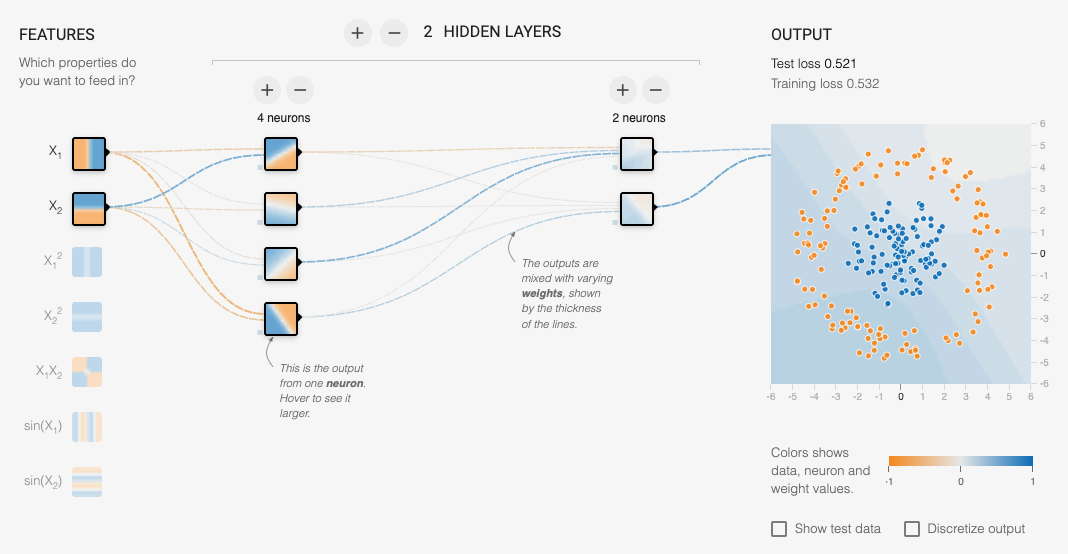
If you are interested to build a more complex neural network, you can try the following website.

The more layers and neurons you add, the more complex the neural network becomes, it can fit more complex data, while in the meantime, it is also more challenging to train.

There are many hyperparameters you can tune in the online playgroud. Explore if we can find the parameters that can fit all the data distributions.

Train a neural network online