How old is the universe?
EPS 88 · PyEarth. Open your own copy on DataHub: click here.
In 1929 nobody knew whether the universe was standing still, shrinking or growing. The astronomer Edwin Hubble compared two measurements for nearby galaxies: how far away each one is, and how fast it is moving away from us. Plotted against each other, the points fell near a straight line: the farther a galaxy, the faster it leaves. That line means the universe is expanding, and its slope says how fast. Run the expansion backwards and every galaxy was once in the same place; the slope tells you how long ago.
Today you repeat Hubble's measurement with much better data: thirty-six exploding stars from a study led by the astronomer Wendy Freedman. You will find the best straight line through them three ways, by guessing, by trying every line and by a formula, then in one line of scikit-learn; check how good the line is; and turn its slope into an age for the universe. At home you try the same method on two more datasets, and find out where a straight line stops working.
Every place you write something opens with a pencil icon and the words Your turn, and is
followed by a cell that already has the shape of the answer written in, with ... wherever your
code goes. Replace every ..., run every cell so your answers and figures are
saved in the file, then download this notebook itself — the .ipynb file — and upload it
to Gradescope. Not a PDF: the marking reads your notebook, and a PDF cannot be read.
In JupyterLab: File ▸ Download, or right-click the file in the left-hand panel and choose
Download.
Two habits from the first minute. A cell runs when you press Shift+Enter, and the notebook remembers everything it has already run — so when something breaks and you cannot see why, Kernel → Restart Kernel and Run All Cells throws the memory away and rebuilds it from the top. That is never the wrong thing to do.
What you'll be able to do
The science. Explain how a plot of speed against distance shows that the universe is expanding, why the best line through it should pass through the origin, and how its slope turns into an age.
The code. A straight line as two numbers, a and b · a residual, and the root mean squared
error that sums them up · a loop that tries many lines · the least-squares formula · scikit-learn:
LinearRegression().fit(x, y), .coef_[0], .intercept_, .predict(x), .score(x, y) and
fit_intercept=False · a function that converts units.
Eleven places where you write something: seven in class, four at home. Each is headed
Your turn, and the cell under it has the shape of the answer written in, with ... wherever
your code goes and a comment beside each one saying what goes there. Early on the comment says
how; later, once you have seen a thing done, it says only what.
The four questions of the class:
- How do we know the universe is expanding?
- How do we find the best straight line?
- What does the best line say about the universe, and how good is it?
- How old does that make the universe?
Setup
Run the next cell once. It loads the three small tables this week uses, all stored with the course: the supernovae for class, and two tables for the homework.
import numpy as np
from sklearn.linear_model import LinearRegression
import pandas as pd
import matplotlib.pyplot as plt

# house style, set once, so every plot cell below holds only what matters
plt.rcParams.update({"figure.dpi": 110,
                     "axes.grid": True, "grid.alpha": 0.3, "axes.axisbelow": True})

CACHE = "https://raw.githubusercontent.com/AI4EPS/EPS88_PyEarth/main/data"

# 36 Type Ia supernovae (Freedman and colleagues, 2001): the three columns to keep are name, speed and distance
supernovae = pd.read_csv(CACHE + "/week06_supernovae.csv")[["Supernova", "VCMB", "D(Mpc)"]]

# For the homework. 21 clusters of galaxies from the same study, with distances measured another way:
clusters = pd.read_csv(CACHE + "/week06_galaxy_clusters.csv")
# and supernovae much farther away (Betoule and colleagues, 2014): redshift, speed and distance
far_supernovae = pd.read_csv(CACHE + "/week06_far_supernovae.csv")[["z", "VCMB", "D(Mpc)"]]

print("supernovae:", len(supernovae), "  galaxy clusters:", len(clusters), "  far supernovae:", len(far_supernovae))
supernovae: 36 galaxy clusters: 21 far supernovae: 31
1. How do we know the universe is expanding?
To test whether the universe is expanding you need two measurements for each galaxy: how fast it is moving away from us, and how far away it is.
Speed comes from colour. You have heard the pitch of a siren drop as a fire engine passes you (listen to one). Sound is a wave, and the length of one wave, from crest to crest, is its wavelength. When the source moves away from you, each new crest starts from a little farther away, so the crests reach you farther apart: the wave arrives stretched. A longer sound wave has a lower pitch (the figure says frequency: fewer waves a second). This is the Doppler effect. In the picture, the car is moving to the right: the person it drives toward gets short waves and a high pitch, the person it leaves behind gets long waves and a low pitch.
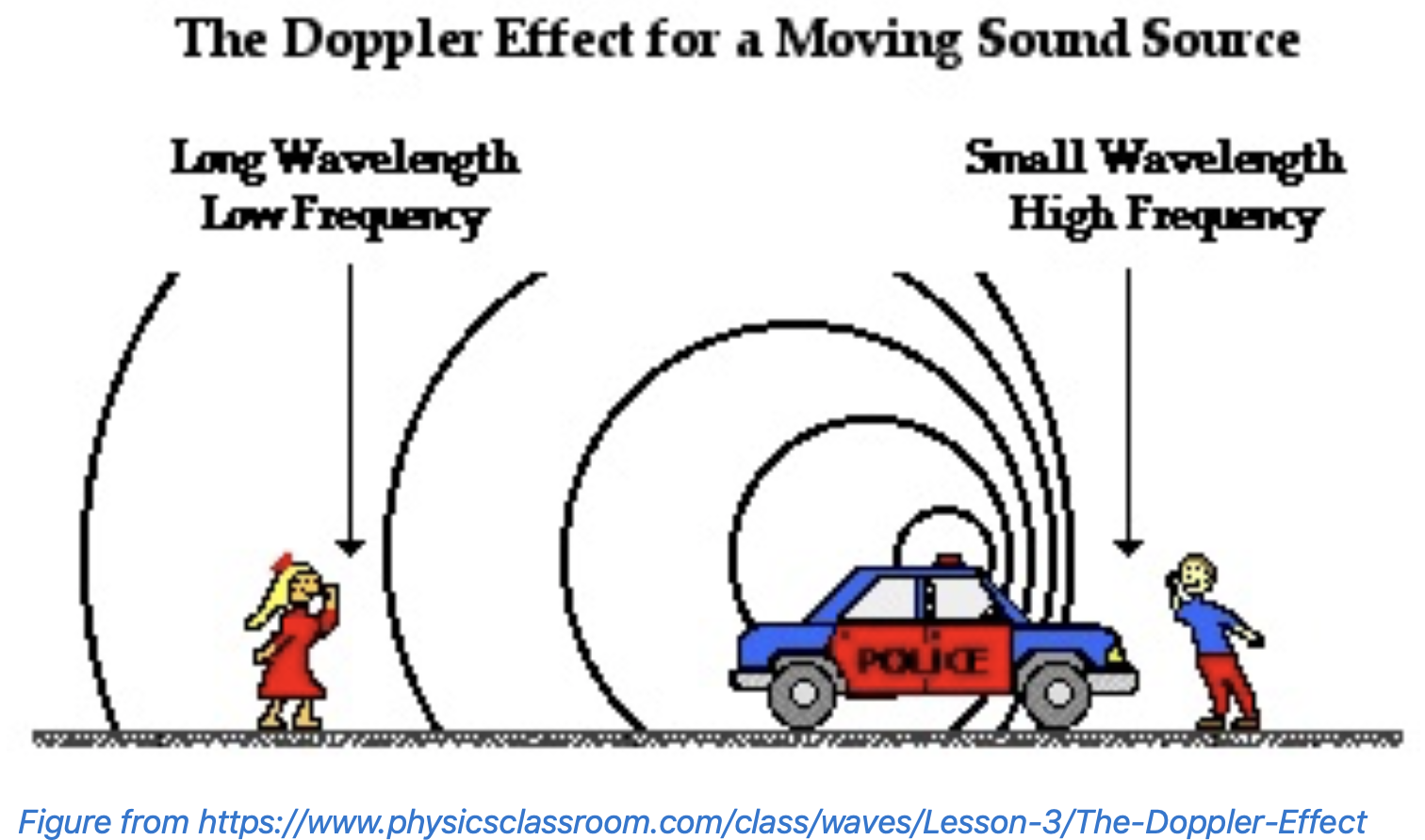
Figure from The Physics Classroom.
Light is a wave too: when a galaxy moves away from us its light arrives with a longer wavelength, and a longer light wave is a redder colour. Astronomers call that a redshift.
How do we know how long the waves were when they left? Hydrogen absorbs light at a few exact wavelengths (measured in nanometres, billionths of a metre), and they show as dark lines in the light of a star: the same pattern everywhere in the universe, like a barcode. In the light of a galaxy that is moving away, the whole barcode sits at longer wavelengths, toward the red end of the rainbow; in the light of one moving toward us, toward the blue:
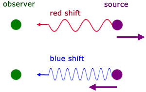
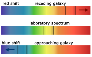
Figures from A-level Physics Tutor.
The size of the shift gives the speed: for speeds well below light's, each wavelength grows by the fraction (the galaxy's speed) / (the speed of light). The fastest galaxy in today's table is leaving at 30,253 km/s, about a tenth of the speed of light, so every one of its lines sits a tenth farther along: hydrogen's red line, at 656 nanometres in a laboratory, arrives at 722. The far-red lines move more than the violet ones, because each one moves by the same fraction of itself: the barcode is stretched, not slid.
Distance comes from brightness. A lamp looks dimmer the farther away it is. So if you know how bright a lamp really is, how bright it looks tells you its distance. Astronomers call such a lamp a standard candle, and a Type Ia supernova is one. It is the explosion of a white dwarf, the small, dense remains of a star, after it has gained matter from a companion star or merged with another white dwarf. These explosions are so alike that astronomers can work out how bright each one really was at its peak. They are also bright enough to be seen in galaxies more than a billion light-years away. Distances that large are measured in megaparsecs (Mpc). One megaparsec is 3.26 million light-years: light, the fastest thing there is, takes 3.26 million years to cross it.
Each row of supernovae is one supernova. VCMB is the speed of its galaxy away from us, in
km/s, with our own motion taken out: the CMB in the name is the cosmic microwave background, the
oldest light in the universe, which astronomers use as the fixed background to measure speeds
against. D(Mpc) is its distance in megaparsecs. That column name has brackets in it, so it
always goes in quotes: supernovae["D(Mpc)"].
supernovae.head()
| Supernova | VCMB | D(Mpc) | |
|---|---|---|---|
| 0 | SN1990O | 9065 | 134.7 |
| 1 | SN1990T | 12012 | 158.9 |
| 2 | SN1990af | 15055 | 198.6 |
| 3 | SN1991S | 16687 | 238.9 |
| 4 | SN1991U | 9801 | 117.1 |
✏️ Your turn 1
Does a galaxy that is farther away move away faster?
Why: if the universe is expanding, speed must grow with distance. A figure of one against the other is the test, and it is the figure Hubble drew.
- The figure. Draw the thirty-six supernovae as a scatter plot, as you did for earthquakes in the plotting week: distance across, speed up, and a label with units on each axis. The dots should climb from the lower left to the upper right.
nearestandfarthest: the smallest and the largest distance in the table. A result holds for the range of its data, so you will need this range later.
Use these names, because the self-check looks for them: nearest and farthest.
plt.figure(figsize=(7, 4))
plt.scatter(supernovae["D(Mpc)"], supernovae["VCMB"])
plt.xlabel("distance (Mpc)")
plt.ylabel("speed away from us (km/s)")
plt.title(f"Type Ia supernovae (n = {len(supernovae)})")
plt.show()

nearest = supernovae["D(Mpc)"].min()
farthest = supernovae["D(Mpc)"].max()
print("the supernovae lie between", nearest, "and", farthest, "Mpc away")

the supernovae lie between 56.0 and 467.0 Mpc away
# Self-check: run this after your answer. You do not need to read it — it only says whether something is off.
assert nearest == 56.0 and farthest == 467.0, "nearest and farthest are the smallest and the largest value of the D(Mpc) column"
print(f"✓ Your turn 1 — the supernovae lie between {nearest} and {farthest} Mpc away")
✓ Your turn 1 — the supernovae lie between 56.0 and 467.0 Mpc away
Farther means faster, and the points fall close to a straight line. Every distant galaxy is moving away from us, and a galaxy twice as far leaves about twice as fast. That is what an expanding universe looks like from inside it. Think of dots drawn on a rubber band, one centimetre apart, and stretch the band to one and a half times its length in one second. Seen from your dot, the dot that was 1 cm away is now at 1.5 cm: it moved 0.5 cm. The dot that was 4 cm away is now at 6 cm: it moved 2 cm, in the same second, so four times as far means four times as fast. Stand on any other dot and you see the same thing. No dot is the centre; the band is simply stretching everywhere.
How fast the universe is expanding is the slope of that line: how many km/s of speed each megaparsec of distance adds. So the measurement you need is the slope of the best straight line through these dots, and section 2 teaches how to find it.
2. How do we find the best straight line?
A straight line is two numbers. Write $y$ for the thing up the page and $x$ for the thing across. Then every straight line is
$$y = a \, x + b$$
$a$ is the slope: how much $y$ grows for each unit of $x$. $b$ is the intercept: the value of $y$ where $x$ is zero, where the line crosses the vertical axis. Choose $a$ and $b$ and you have chosen the line. Finding the best line through a cloud of points means choosing the best pair. This section finds it for the supernovae three ways, each better than the last: by guessing, by trying every pair, and by a formula. Then scikit-learn does it in one line.
✏️ Your turn 2
Guess the line.
Why: before any formula, see what a slope and an intercept do to a line, and how far a guess can be from the data. Four guesses of your own, drawn on the dots, show it.
draw_line(a, b): a function that draws the line $y = a\,x + b$ from 0 to 500 Mpc onto whatever figure is open. Its body is one drawing call: a line needs only its two end points, at $x = 0$ and $x = 500$, whichline_xholds, and its two speeds area * line_x + b. The label names the pair, so the legend tells the lines apart.guesses: four pairs of your own, each a list[a, b]. From Your turn 1, the speeds reach about 30,000 km/s at 470 Mpc, so slopes between 40 and 100 are worth trying, and intercepts between −5,000 and 5,000.- The figure: the supernovae as dots, then the loop calls your function once per pair, so all four lines land on the same dots. Which looks best? Which is too flat, and which starts in the wrong place?
Use these names, because the self-check looks for them: draw_line and guesses.
line_x = np.array([0, 500])                     # the two ends of the line, in Mpc


def draw_line(a, b):
    """the line y = a x + b, from 0 to 500 Mpc, on the figure that is open"""
    plt.plot(line_x, a * line_x + b, label=f"a = {a}, b = {b}")


guesses = [[50, 0], [85, 2000], [70, -3000], [65, 1500]]

plt.figure(figsize=(7, 4))
plt.scatter(supernovae["D(Mpc)"], supernovae["VCMB"], color="black", s=12, label="supernovae")
for guess in guesses:                           # one line for each pair, on the same dots
    draw_line(guess[0], guess[1])
plt.xlabel("distance (Mpc)")
plt.ylabel("speed away from us (km/s)")
plt.legend()
plt.title("Four guessed lines")
plt.show()

# Self-check: run this after your answer. You do not need to read it — it only says whether something is off.
assert callable(draw_line) and draw_line.__code__.co_argcount == 2, "draw_line is a function of two numbers, a slope and an intercept"
assert len(guesses) == 4, "guesses holds four pairs"
for guess in guesses:
    assert len(guess) == 2 and -200 < guess[0] < 200 and -20000 < guess[1] < 20000, "each guess is a list of two numbers, a slope then an intercept, within reason"
print(f"✓ Your turn 2 — four lines drawn; the next cells say which one is best")
✓ Your turn 2 — four lines drawn; the next cells say which one is best
Judging by eye is not enough. Two guesses that both look close cannot be told apart by looking. To choose between them you need a number that says how badly a line misses its points.
A residual is the real value minus the line's value.
$$\text{residual} = \text{real value} - \text{the line's value}$$
Take the first supernova in the table, SN1990O, 134.7 Mpc away at 9,065 km/s, and a reasonable guess, $a = 72$ and $b = 300$. The line gives it $72 \times 134.7 + 300 = 9,998$ km/s. Its residual for that line is $9,065 - 9,998 = -933$ km/s: the point sits that far below the line. A point above the line has a positive residual.
To judge a whole line with one number, use the root mean squared error, RMSE. A line has thirty-six residuals. Square each one, so that misses above and below the line cannot cancel; take the mean of the squares; take the square root, which brings the number back to km/s:
$$\text{RMSE} = \sqrt{\text{mean of the squared residuals}}$$
The RMSE is the typical miss of the line, in the units of the data. Try it on three residuals,
2, −2 and 1. Added as they are they give 1, as if the line hardly missed. Their squares are 4, 4
and 1, the mean is 3, and the square root of 3 is 1.7. In Python the square root
is a power of one half: (mean) ** 0.5. Squaring makes a line care most about its worst misses;
the number a fit tries to make small is also called its loss. The next cell scores your four
guesses, and the example line.
for guess in guesses + [[72, 300]]:      # your four pairs, then the example line
    a = guess[0]
    b = guess[1]
    guess_residuals = supernovae["VCMB"] - (a * supernovae["D(Mpc)"] + b)   # real speed minus the line's, one per supernova
    guess_rmse = ((guess_residuals ** 2).mean()) ** 0.5                     # square, average, square root
    print("a =", a, " b =", b, "  RMSE =", round(guess_rmse), "km/s")
a = 50  b = 0   RMSE = 4278 km/s
a = 85  b = 2000   RMSE = 4787 km/s
a = 70  b = -3000   RMSE = 3413 km/s
a = 65  b = 1500   RMSE = 1028 km/s
a = 72  b = 300   RMSE = 1099 km/s
The smallest RMSE wins; the example line misses by 1,099 km/s. But a better pair may exist that nobody guessed. The way to find it is to stop guessing and try every pair.
✏️ Your turn 3
Try every line.
Why: the best line is the one with the smallest RMSE. A loop inside a loop can try every
whole slope from 50 to 90 and every intercept from −3,000 to 3,000 in steps of 100, and keep
three lists: each RMSE, and the a and b that made it. That is 2,501 lines in a second, and
the smallest RMSE in the list is the best line.
- Inside the loops: for each
band eacha, the residuals and the RMSE, as in the cell above, then append the RMSE tormses, andaandbtoslopesandintercepts, so that the three lists line up. lowest,where,best_aandbest_b: the smallest RMSE withnp.min, its position inrmseswithnp.argmin, and the slope and intercept at that same position in the other two lists, as you read one list by the position found in another in the first week.- The rest is given: the 2,501 RMSEs reshaped into a grid, one row per intercept, and drawn as a picture, as the elevation week drew a grid, with your guesses as dots and the best pair as a star.
Use these names, because the self-check looks for them: rmse_grid, lowest, best_a and
best_b.
a_values = np.arange(50, 91)                    # every whole slope from 50 to 90
b_values = np.arange(-3000, 3001, 100)          # every intercept from -3,000 to 3,000, in steps of 100
rmses = []                                      # one RMSE per line tried
slopes = []                                     # the a of that line
intercepts = []                                 # and its b
for b in b_values:
    for a in a_values:
        residuals = supernovae["VCMB"] - (a * supernovae["D(Mpc)"] + b)
        rmse = ((residuals ** 2).mean()) ** 0.5
        rmses.append(rmse)
        slopes.append(a)
        intercepts.append(b)

lowest = np.min(rmses)
where = np.argmin(rmses)
best_a = slopes[where]
best_b = intercepts[where]
rmse_grid = np.array(rmses).reshape(len(b_values), len(a_values))  # the same numbers as a grid: one row per intercept, one column per slope

plt.figure(figsize=(7, 4.2))
plt.imshow(rmse_grid, extent=[50, 90, -3000, 3000], origin="lower", aspect="auto", cmap="Blues_r", vmax=3000)
plt.colorbar(label="RMSE (km/s)")
for guess in guesses:                           # your guesses, where they fall on the map
    plt.scatter(guess[0], guess[1], color="black")
plt.scatter(best_a, best_b, color="red", marker="*", s=180, label=f"the best pair: a = {best_a}, b = {best_b}")
plt.xlabel("a, the slope (km/s per Mpc)")
plt.ylabel("b, the intercept (km/s)")
plt.legend(loc="lower left", fontsize=8)
plt.title("The RMSE of every line: dark is good; black dots are your guesses")
plt.show()

print("the best pair: a =", best_a, " b =", best_b, "  RMSE =", round(lowest), "km/s")

the best pair: a = 67 b = 800 RMSE = 943 km/s
# Self-check: run this after your answer. You do not need to read it — it only says whether something is off.
assert len(rmses) == len(slopes) == len(intercepts) == 2501, "the three lists must line up: one RMSE, one a and one b appended for every line tried"
assert abs(rmse_grid[30, 20] - 1007.3) < 2, "the RMSE of a = 70, b = 0 must come out as in the cell above: residuals squared, averaged, then ** 0.5"
assert abs(lowest - 943) < 2, "lowest is the smallest RMSE: np.min(rmses)"
assert best_a == 67 and best_b == 800, "best_a and best_b are the slope and the intercept at the position of lowest: where = np.argmin(rmses), then slopes[where] and intercepts[where]"
print(f"✓ Your turn 3 — of 2,501 lines, a = {best_a} and b = {best_b} miss least, by {round(lowest):,} km/s")
✓ Your turn 3 — of 2,501 lines, a = 67 and b = 800 miss least, by 943 km/s
The picture is a valley. Every pair in the dark band is a good line, and the band runs diagonally: a steeper line can be made nearly as good by starting it lower. The lowest point is $a = 67$, $b = 800$, with an RMSE of 943 km/s. Finding it this way is called least squares: the line with the smallest RMSE is the line with the smallest total of squared residuals, the same thing.
Trying every pair works, but it is slow and it only finds pairs on the grid. For a straight line there is a formula that goes to the bottom of the valley directly.
The formula. Call the distances $x_1, \ldots, x_n$ and the speeds $y_1, \ldots, y_n$, with $n = 36$, and let $\bar{x}$ and $\bar{y}$ be their averages. The $a$ and $b$ with the smallest RMSE are
$$a = \frac{\sum (x_i - \bar{x})(y_i - \bar{y})}{\sum (x_i - \bar{x})^2}, \qquad b = \bar{y} - a\,\bar{x}$$
The top of $a$ adds up, over the points, how far each one is from the average in $x$ times how far it is in $y$: positive when the two go together. The bottom is how spread out the $x$ are. And $b$ makes the line pass through the point of averages, $(\bar{x}, \bar{y})$. Proving that this pair is the bottom of the valley takes calculus; the next cell checks it instead.
✏️ Your turn 4
The formula, by hand.
Why: a formula you have applied once is one you can trust, and the loop gives you the answer to check it against.
x_from_meanandy_from_mean: how far each distance is from the average distance, and each speed from the average speed. One line each, on the whole column.a_by_hand: the top of the formula over its bottom: the two columns multiplied and summed, over the squared distances-from-mean summed.b_by_hand: the average speed minusa_by_handtimes the average distance.
The print sets your two numbers beside best_a and best_b, the best pair the loop found in
Your turn 3.
Use these names, because the self-check looks for them: a_by_hand and b_by_hand.
x_from_mean = supernovae["D(Mpc)"] - supernovae["D(Mpc)"].mean()
y_from_mean = supernovae["VCMB"] - supernovae["VCMB"].mean()
a_by_hand = (x_from_mean * y_from_mean).sum() / (x_from_mean ** 2).sum()
b_by_hand = supernovae["VCMB"].mean() - a_by_hand * supernovae["D(Mpc)"].mean()

print("by the formula: a =", round(a_by_hand, 1), " b =", round(b_by_hand))
print("by the loop:    a =", best_a, " b =", best_b)
by the formula: a = 67.5  b = 712
by the loop:    a = 67  b = 800
# Self-check: run this after your answer. You do not need to read it — it only says whether something is off.
assert abs(a_by_hand - 67.5362) < 0.05, "a_by_hand is sum((x - mean x) * (y - mean y)) over sum((x - mean x) ** 2)"
assert abs(b_by_hand - 711.8) < 5, "b_by_hand is the average speed minus a_by_hand times the average distance"
print(f"✓ Your turn 4 — the formula gives a = {round(a_by_hand, 1)} and b = {round(b_by_hand)}")
✓ Your turn 4 — the formula gives a = 67.5 and b = 712
The formula lands at $a = 67.5$, $b = 712$, inside the grid square the loop found; the loop could only land on whole slopes and intercepts in steps of 100. The RMSE of the formula's line is the smallest any straight line can have on these points.
scikit-learn does the formula in one line. That is linear regression: draw the best straight line. Best means the smallest root mean squared error: the line that misses its points least.
scikit-learn is Python's library of methods that learn from data. You will use it in most weeks from now on, and every method in it works in the same three steps:
| step | code | what it does |
|---|---|---|
| make a model | LinearRegression() |
a rule with numbers still to choose: here $y = a\,x + b$, with $a$ and $b$ unknown. Machine learning calls the numbers parameters |
| fit it | .fit(x, y) |
chooses the numbers from the data by making the RMSE as small as it can: for a line, the formula above. Machine learning calls that training |
| ask it | .predict(x) |
applies the rule to any x |
Two different things happen in LinearRegression().fit(x, y). LinearRegression() makes the
model: an empty one, with no $a$ and no $b$, because it has seen no data. .fit(x, y) gives it
the data; the model chooses its two numbers and keeps them. fit also hands the fitted model
back, which is why the two steps can sit on one line. In the next cell you do them one at a
time, once, to see the difference.
x must be a table, because a fit can use several columns at once. supernovae["D(Mpc)"], one
pair of brackets, is a single column. supernovae[["D(Mpc)"]], two pairs, is a table of one
column, and that is what fit wants. y is the column to predict. LinearRegression came from
the setup cell: from sklearn.linear_model import LinearRegression imports one method by name
from a large library.
| In the equations | In scikit-learn |
|---|---|
| $x$, $y$ | the two arguments of .fit(x, y): x as a one-column table, y a column |
| $a$, the slope | model.coef_[0]: one slope for each column of x, so take the first |
| $b$, the intercept | model.intercept_ |
| $y = a\,x + b$ at any $x$ | model.predict(x) |
| the $a$, $b$ with the smallest RMSE | what .fit chooses, by the formula |
| $b$ held at zero, so the line passes through the origin | LinearRegression(fit_intercept=False) (section 3) |
| $R^2$, how good the line is | model.score(x, y) (section 3) |
The underscore at the end of coef_ and intercept_ marks a number the fit chose.
3. What does the best line say about the universe, and how good is it?
Section 2 was the method, and you now know what scikit-learn does when it fits a line. From here on the notebook uses it directly and reads the science off the line: its slope is a measurement, its intercept is fixed by the physical model, and its residuals say how far to trust it.
✏️ Your turn 5
Fit the supernovae with scikit-learn, and use the line.
Why: this is the call you will make in every later week. Its two numbers should match the
formula (a_by_hand, b_by_hand) and the loop (best_a, best_b), and a fitted line can
give a speed at a distance where nothing was measured.
model: the first two lines make the empty model and print it; then fit it: distance asx, as a one-column table, and speed asy.slopeandintercept: the two numbers of the line, read from the model.line_speed: the line's speed at each supernova's distance, frommodel.predict.speed_350: the speed the rule gives a galaxy 350 Mpc away: speed = slope × 350 + intercept. No supernova is at that distance, but it is inside the range of the table.- The figure, three things on it: the supernovae as dots, the line on top in black, and
your prediction as one red cross at distance 350. The line should run through the middle of
the dots, and the cross should sit on it. Remember the difference:
plt.scatterdraws one dot per row and joins nothing;plt.plotjoins its points in order into a line. Every value ofline_speedlies on the same straight line, so the order of the rows does not matter.
Two errors to expect: Expected a 2-dimensional container means the distance needs its second
pair of brackets; doesn't define __round__ means the slope needs its [0].
Use these names, because the self-check looks for them: model, slope, intercept,
line_speed and speed_350.
model = LinearRegression()                      # make: an empty model, with no a or b yet
print("before fit:", model)                     # it prints as just its name: it holds no numbers
model.fit(supernovae[["D(Mpc)"]], supernovae["VCMB"])
slope = model.coef_[0]
intercept = model.intercept_
line_speed = model.predict(supernovae[["D(Mpc)"]])
speed_350 = slope * 350 + intercept

plt.figure(figsize=(7, 4))
plt.scatter(supernovae["D(Mpc)"], supernovae["VCMB"], label="supernovae")
plt.plot(supernovae["D(Mpc)"], line_speed, color="black", label="the best straight line")
plt.scatter(350, speed_350, color="red", marker="x", s=90, label="your prediction at 350 Mpc")
plt.xlabel("distance (Mpc)")
plt.ylabel("speed away from us (km/s)")
plt.legend()
plt.title(f"The best straight line through {len(supernovae)} supernovae")
plt.show()

print("by scikit-learn: a =", round(slope, 1), " b =", round(intercept))
print("by the formula:  a =", round(a_by_hand, 1), " b =", round(b_by_hand))
print("by the loop:     a =", best_a, " b =", best_b)
print("a galaxy 350 Mpc away leaves at", round(speed_350), "km/s")
before fit: LinearRegression()

by scikit-learn: a = 67.5  b = 712
by the formula:  a = 67.5  b = 712
by the loop:     a = 67  b = 800
a galaxy 350 Mpc away leaves at 24349 km/s
# Self-check: run this after your answer. You do not need to read it — it only says whether something is off.
assert 67 < model.coef_[0] < 68 and 700 < model.intercept_ < 725, "model is fitted to distance (two pairs of brackets) as x and speed as y: model.fit(...)"
assert isinstance(slope, float), "slope is one number: model.coef_ holds one slope for each column of x, so take the first, with [0]"
assert abs(slope - model.coef_[0]) < 0.06 and abs(intercept - model.intercept_) < 1, "slope is model.coef_[0] and intercept is model.intercept_"
assert len(line_speed) == len(supernovae) and abs(line_speed - model.predict(supernovae[["D(Mpc)"]])).max() < 25, "line_speed is model.predict on the distances, as a one-column table"
assert abs(speed_350 - (model.coef_[0] * 350 + model.intercept_)) < 30, "speed_350 is slope times 350, plus intercept"
print(f"✓ Your turn 5 — slope {round(slope, 1)} km/s per Mpc, intercept {round(intercept)} km/s, and {round(speed_350)} km/s at 350 Mpc")
✓ Your turn 5 — slope 67.5 km/s per Mpc, intercept 712 km/s, and 24349 km/s at 350 Mpc
The fitted line has a slope of 67.5 km/s per Mpc: your first measurement of the Hubble constant. For every megaparsec farther away, a galaxy leaves 67.5 km/s faster.
Now compare your prediction with the table. No supernova is at 350 Mpc, but the table holds some on each side of it. Before anyone had a line, this was how a prediction was made: take the neighbours and average them. A line does the same job with one rule for every distance, including distances where there are no neighbours at all. The cell lists the supernovae between 300 and 400 Mpc; your figure above shows the prediction as the red cross among them.
near_350 = supernovae[(supernovae["D(Mpc)"] > 300) & (supernovae["D(Mpc)"] < 400)]  # the supernovae between 300 and 400 Mpc
print(near_350.sort_values("D(Mpc)"))                                              # nearest first
print("your line at 350 Mpc:", round(speed_350), "km/s")
   Supernova   VCMB  D(Mpc)
22   SN1993B  21190   303.4
19  SN1992bp  23646   309.5
20  SN1992br  26318   391.5
your line at 350 Mpc: 24349 km/s
Think. SN1992bp, at 309.5 Mpc, leaves at 23,646 km/s, and SN1992br, at 391.5 Mpc, at 26,318 km/s. Your line gives 24,349 km/s at 350 Mpc, between the two. Why is it reasonable to trust the line here? Would you trust it as much at 3,500 Mpc, far beyond the last supernova? The homework tests that.
The slope is the Hubble constant, and the physical model has no intercept. In 1929 Hubble wrote the line through these dots as a law:
$$v = H_0 \, d$$
where $v$ is a galaxy's speed, $d$ its distance, and $H_0$ the Hubble constant: how fast the universe is expanding now, in km/s per Mpc. Your slope, 67.5, is a measurement of $H_0$. The law has no intercept: at $d = 0$ it gives $v = 0$. The galaxy at zero distance is our own, and a galaxy cannot move away from itself, so in this model the line passes through the origin. Your free fit chose an intercept of 712 km/s because nothing told it not to; read literally, that would say our own galaxy is moving away from itself.
The free fit is still useful, as a check on the data: against speeds of tens of thousands of km/s, 712 is close to zero, so the supernovae are consistent with a line through the origin, as the law says.
Fit the line the physical model gives. When the physical model fixes a point on the line, the fit keeps it. In scikit-learn that is one argument, given when the model is made:
LinearRegression(fit_intercept=False).fit(x, y)
fit_intercept=False tells the model not to choose an intercept: $b$ is held at zero, and the
fit chooses only $a$. Everything else is the same three steps, and .coef_[0] is still the
slope. You will fit that line in section 4. First, how good is the free line?
✏️ Your turn 6
How well does the line fit the supernovae?
Why: a line can be the best one and still be the wrong shape for its data. Two things tell you: a picture, the residual plot, the residuals drawn against distance; and one number, R².
R² compares your line with the simplest line there is, a flat one at the average speed, which ignores distance altogether:
$$R^2 = 1 - \left(\frac{\text{RMSE of the fitted line}}{\text{RMSE of the flat line}}\right)^2$$
It is 1 when every point sits on the line, and near 0 when the line does no better than the average. The flat line is the yardstick; it has no R² of its own here.
residuals: the real speed minusline_speed, one for each supernova.- The figure: the residuals against distance, as dots, with a horizontal line at zero to
measure from.
plt.axhline(0)draws one. line_rmse: the RMSE of the fitted line, as in section 2.flat_rmse: the RMSE of a flat line at the average speed: the residuals of that line are each speed minus the average speed.r_squared: by the equation, from the two RMSEs. The last line asks scikit-learn for the same number withmodel.score(x, y), which takes the same two things the fit was given.
Use these names, because the self-check looks for them: residuals, line_rmse, flat_rmse
and r_squared.
residuals = supernovae["VCMB"] - line_speed

plt.figure(figsize=(7, 4))
plt.scatter(supernovae["D(Mpc)"], residuals)
plt.axhline(0, color="black")
plt.xlabel("distance (Mpc)")
plt.ylabel("residual: real speed minus the line's (km/s)")
plt.title(f"What the line misses (n = {len(supernovae)})")
plt.show()

line_rmse = ((residuals ** 2).mean()) ** 0.5
flat_rmse = (((supernovae["VCMB"] - supernovae["VCMB"].mean()) ** 2).mean()) ** 0.5
r_squared = 1 - (line_rmse / flat_rmse) ** 2

print("the fitted line misses by", round(line_rmse), "km/s; a flat line at the average speed by", round(flat_rmse))
print("R² by the equation:", round(r_squared, 3), "   R² from model.score, the same number:", round(model.score(supernovae[["D(Mpc)"]], supernovae["VCMB"]), 3))

the fitted line misses by 942 km/s; a flat line at the average speed by 6391
R² by the equation: 0.978    R² from model.score, the same number: 0.978
# Self-check: run this after your answer. You do not need to read it — it only says whether something is off.
assert 3069 < residuals.max() < 3269 and -2098 < residuals.min() < -1898, "residuals is the real speed minus line_speed, in that order"
assert abs(line_rmse - ((residuals ** 2).mean()) ** 0.5) < 1, "line_rmse is the square root of the MEAN of the SQUARED residuals: square, average, ** 0.5"
assert abs(flat_rmse - 6391) < 2, "flat_rmse is the RMSE of the residuals from the AVERAGE speed: speed minus the mean, squared, averaged, ** 0.5"
assert abs(r_squared - model.score(supernovae[["D(Mpc)"]], supernovae["VCMB"])) < 0.002, "r_squared is 1 minus (line_rmse / flat_rmse) squared"
print(f"✓ Your turn 6 — the line misses by {round(line_rmse):,} km/s, the flat line by {round(flat_rmse):,}, so R² is {round(r_squared, 3)}")
✓ Your turn 6 — the line misses by 942 km/s, the flat line by 6,391, so R² is 0.978
R² is 0.978. The line's RMSE is about 15 percent of the flat line's, and R² works with the squares, so the line leaves about 2 percent of the flat line's squared miss. One thing to notice: the flat line's residuals are the distances of the speeds from their average, so its RMSE is the standard deviation of the speeds, the measure of spread from the probability week.
The residual plot of a good fit shows no pattern: the points lie on both sides of zero all the way across. A pattern is a tilt or a curve, and it means a straight line is the wrong shape, however high R² is. A second thing to look for is the scatter growing wider from one end to the other: the line is still the best straight line, but less sure at the wide end. Your plot shows no tilt or curve, a little widening toward the far end, and the two farthest supernovae below the line, a first hint of what you meet in the homework. Between 56.0 and 467.0 Mpc a straight line is a good description of these data. The universe is expanding, and you have measured how fast.
What R² looks like. R² is the square of the correlation coefficient $r$, a number between −1 and 1. The top row of the gallery shows clouds of points with $r$ from 1 (a perfect line going up) through 0 (no relation) to −1 (a perfect line going down). The middle row says that $r$ does not care how steep the line is: a perfect line gives 1 or −1 whatever its slope, and a flat line has no $r$ at all. The bottom row is the warning: in every one of those shapes $x$ and $y$ are clearly related, yet $r$ is 0, because the relation is not a straight line. R² cannot see that. The residual plot can.
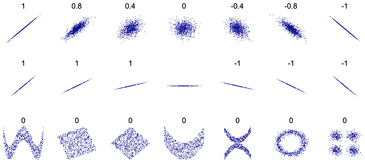
Figure from Wikipedia, Correlation and dependence.
4. How old does that make the universe?
This section uses slope from Your turn 5; run that cell again if you restarted.
A friend arrives at your door and says: "I drove 120 km at 60 km/h." You know when your friend left: 120 divided by 60, two hours ago. Time is distance divided by speed. The same works for a galaxy. If it has always moved at the speed it has today, the time since it was right here is
$$t = \frac{d}{v}$$
Hubble's law says $v = H_0 d$. Put that in, and the distance cancels:
$$t = \frac{d}{H_0 \, d} = \frac{1}{H_0}$$
The same time for every galaxy, near or far: they all set out together. So one over the slope is an age for the universe.
one_over_slope = 1 / slope
print("one over the slope:", round(one_over_slope, 4), "Mpc·s/km")
one over the slope: 0.0148 Mpc·s/km
A small number in an unfamiliar unit. The slope is in km/s per Mpc. One over it turns the unit upside down: Mpc per (km/s), which is megaparsec-seconds per kilometre, written Mpc·s/km. It is a time, written as a length divided by a speed. Three steps turn it into years, one unit at a time.
Step 1: a megaparsec is $3.0857 \times 10^{19}$ km. Multiply by that, and the Mpc cancels the Mpc while the km cancels the km, leaving seconds:
$$0.0148\ \frac{\text{Mpc}\cdot\text{s}}{\text{km}} \times 3.0857 \times 10^{19}\ \frac{\text{km}}{\text{Mpc}} = 4.57 \times 10^{17}\ \text{s}$$
Step 2: a year has $60 \times 60 \times 24 \times 365.25 = 31,557,600$ seconds. Divide by that, and the seconds cancel, leaving years:
$$\frac{4.57 \times 10^{17}\ \text{s}}{31,557,600\ \text{s/year}} = 1.45 \times 10^{10}\ \text{years}$$
Step 3: divide by a billion, $10^9$, to get 14.48 billion years.
Python writes such numbers with an e for "times ten to the": 3.0857e19 is
$3.0857 \times 10^{19}$, 1e9 is a billion, and a result that prints as 4.57e+17 means
$4.57 \times 10^{17}$. The next cell does the three steps.
MPC_IN_KM = 3.0857e+19                     # kilometres in one megaparsec: 3.0857 × 10^19, written with an e
age_seconds = one_over_slope * MPC_IN_KM    # step 1: Mpc·s/km × km/Mpc leaves seconds
print("step 1:", age_seconds, "seconds")    # printed as 4.57e+17: 4.57 × 10^17 seconds

SECONDS_PER_YEAR = 60 * 60 * 24 * 365.25    # seconds in a minute × minutes in an hour × hours in a day × days in a year
age_years = age_seconds / SECONDS_PER_YEAR  # step 2: seconds ÷ seconds per year leaves years
print("step 2:", f"{round(age_years):,}", "years")   # :, puts commas in the thousands

age_billions = age_years / 1e9              # step 3: years ÷ a billion
print("step 3:", round(age_billions, 2), "billion years")
step 1: 4.56895805984196e+17 seconds
step 2: 14,478,154,422 years
step 3: 14.48 billion years
About 14.48 billion years, from the free line. But section 3 said the line to keep is the one through the origin, with no intercept, and it has a different slope. You need the age for that line too, and the homework brings more slopes. A function does the conversion once, for any slope.
✏️ Your turn 7
Write the conversion once, as a function, and use it on both lines.
Why: you now have two lines, and the homework brings more. A function does the three steps in one call, for any slope.
age_of_universe(hubble_constant): it takes a Hubble constant in km/s per Mpc and returns one over it, in billions of years. Its body is the three steps of the cell above, withhubble_constantin place ofslope, and it ends withreturn, as your functions in the functions week did. The two constants are written again inside the function, so that it needs nothing from outside.age: call the function on yourslope, the free line's.origin_modelandH0_origin: fit the line through the origin, withfit_intercept=Falseas section 3 showed, and read its slope.age_origin: call the function onH0_origin.
Use these names, because the self-check looks for them: age_of_universe, age,
origin_model, H0_origin and age_origin.
def age_of_universe(hubble_constant):
    """one over a Hubble constant in km/s per Mpc, as an age in billions of years"""
    MPC_IN_KM = 3.0857e+19  # kilometres in one megaparsec
    SECONDS_PER_YEAR = 60 * 60 * 24 * 365.25
    seconds = (1 / hubble_constant) * MPC_IN_KM
    years = seconds / SECONDS_PER_YEAR
    return years / 1e9


age = age_of_universe(slope)
print("the free line:", round(slope, 2), "km/s per Mpc gives", round(age, 2), "billion years")

origin_model = LinearRegression(fit_intercept=False).fit(supernovae[["D(Mpc)"]], supernovae["VCMB"])
H0_origin = origin_model.coef_[0]
age_origin = age_of_universe(H0_origin)
print("the line through the origin:", round(H0_origin, 2), "km/s per Mpc gives", round(age_origin, 2), "billion years")
the free line: 67.54 km/s per Mpc gives 14.48 billion years
the line through the origin: 70.67 km/s per Mpc gives 13.84 billion years
# Self-check: run this after your answer. You do not need to read it — it only says whether something is off.
assert age_of_universe(70) is not None, "end the function with return, not with print"
assert 13.9 < age_of_universe(70) < 14.1 and 19.4 < age_of_universe(50) < 19.7, "the age must come from the value handed to the function: 70 gives about 14 billion years and 50 about 19.6"
assert abs(age - age_of_universe(slope)) < 0.01, "age is age_of_universe called on your slope"
assert origin_model.intercept_ == 0 and 70.5 < origin_model.coef_[0] < 70.9, "origin_model is fitted with fit_intercept=False to the supernovae: distance as a one-column table, then speed"
assert isinstance(H0_origin, float) and abs(H0_origin - origin_model.coef_[0]) < 0.01, "H0_origin is the slope of origin_model: origin_model.coef_[0]"
assert abs(age_origin - age_of_universe(H0_origin)) < 0.01, "age_origin is age_of_universe called on H0_origin"
print(f"✓ Your turn 7 — {round(age, 2)} billion years from the free line, {round(age_origin, 2)} from the line through the origin")
✓ Your turn 7 — 14.48 billion years from the free line, 13.84 from the line through the origin
The two lines give two ages. The next cell draws them on the data and compares how badly each misses.
origin_residuals = supernovae["VCMB"] - origin_model.predict(supernovae[["D(Mpc)"]])
origin_rmse = ((origin_residuals ** 2).mean()) ** 0.5   # how badly the line through the origin misses
ends = pd.DataFrame({"D(Mpc)": [0, 500]})    # two distances, zero and just past the farthest supernova: enough to draw a straight line
free_ends = model.predict(ends)                 # the free line's speed at those two distances
origin_ends = origin_model.predict(ends)        # and the speed of the line through the origin

plt.figure(figsize=(7, 4))
plt.scatter(supernovae["D(Mpc)"], supernovae["VCMB"], s=12, label="supernovae")
plt.plot(ends["D(Mpc)"], free_ends, color="black", label="the free line")
plt.plot(ends["D(Mpc)"], origin_ends, color="red", ls="--", label="the line through the origin")
plt.xlabel("distance (Mpc)")
plt.ylabel("speed away from us (km/s)")
plt.legend()
plt.title("Two lines through the same supernovae")
plt.show()

print("the free line:          ", round(slope, 2), "km/s per Mpc, so", round(age, 2), "billion years;  RMSE 942 km/s (Your turn 6)")
print("the line through origin:", round(H0_origin, 2), "km/s per Mpc, so", round(age_origin, 2), "billion years;  RMSE", round(origin_rmse), "km/s")

the free line:           67.54 km/s per Mpc, so 14.48 billion years;  RMSE 942 km/s (Your turn 6)
the line through origin: 70.67 km/s per Mpc, so 13.84 billion years;  RMSE 998 km/s
The two lines are hard to tell apart over the data, and they still differ by more than half a billion years: 14.48 against 13.84. The free line misses these thirty-six points slightly less (942 against 998 km/s). The free fit was not wrong: it had no information about where the line starts. The physical model supplies that, and the slope changes with it. The line through the origin is the one to keep: a Hubble constant of 70.7 km/s per Mpc.
Part of the free line's intercept may be real. The two farthest supernovae lie a little below a straight line from zero. A free line tilts down to meet them, and a flatter line starts higher. Two points of thirty-six cannot settle it; the homework looks at that bend, much farther away.
Astronomers are still measuring this number. Here are two recent results: one from the Planck satellite, which mapped the oldest light in the universe, and one from Wendy Freedman's group, which used stars and supernovae as standard candles.
age_planck = age_of_universe(67.4)
age_freedman = age_of_universe(69.8)
print("Planck satellite, 2018:         H0 = 67.4, so 1/H0 =", round(age_planck, 2), "billion years")
print("Freedman and colleagues, 2019:  H0 = 69.8, so 1/H0 =", round(age_freedman, 2), "billion years")
Planck satellite, 2018:         H0 = 67.4, so 1/H0 = 14.51 billion years
Freedman and colleagues, 2019:  H0 = 69.8, so 1/H0 = 14.01 billion years
Three ways to measure the Hubble constant, and they do not agree. The figure below, from Wendy Freedman's group, shows every published value from 2001 to 2019. Each dot is one measurement, its bar is the uncertainty the authors gave, and the shaded band joins the results of one method over the years. The three methods:
| method | colour | how it works | value today |
|---|---|---|---|
| Cepheids | blue | stars that pulse at a rate set by their true brightness: a standard candle, like the supernovae, so a distance and a speed, as in this notebook | about 74 |
| CMB | black | the cosmic microwave background, the oldest light in the universe, released 380,000 years after the start: the pattern of its hot and cold spots, put through a model of the expansion, gives H₀. The Planck value, 67.4, is the last black dot | about 67 |
| TRGB | red | the tip of the red giant branch: the brightest red giant stars all have the same true brightness, so they are a second standard candle. Freedman's own result, 69.8, is the red star | about 70 |
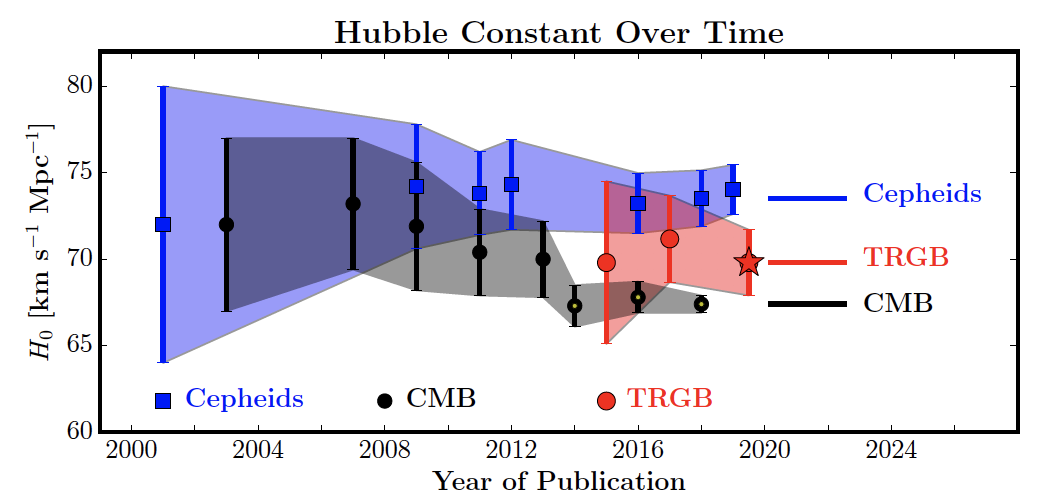
Figure from Freedman et al. (2019), arXiv:1907.05922.
How to read the figure. In 2001 every bar was wide and they all overlapped, so the methods agreed. By 2016 the bars had shrunk, and the blue and the black no longer overlap: two careful methods give values 7 percent apart, more than their uncertainties allow. That disagreement is the Hubble tension. Either one method has an error nobody has found, or the model of the expansion that the CMB value relies on is missing something. It is one of the open questions of astronomy today, and Freedman explains it in this short video.
Why the published age is 13.8 billion years and not 1/H₀. Your calculation assumed that every galaxy has always moved at the speed it has today. That is the friend who drove 120 km at a steady 60 km/h. If the friend drove slowly at first and fast at the end, "two hours ago" is only an estimate.
The universe did both. For the first several billion years gravity slowed the expansion down. Since then it has been speeding up again, pushed by something astronomers call dark energy and do not yet understand. The published age comes from a model of that whole history, not from today's speed alone. The slowing and the speeding-up nearly cancel, which is why 1/H₀ lands within about 5 percent of 13.8: the right size, but not the exact age.
The question, answered
About 14 billion years. One over the slope of the best straight line through thirty-six supernovae gives 13.84 billion years when the line starts at zero, as Hubble's law says it must. The published age, from a model of the whole expansion, is 13.8 billion years. The close agreement is partly luck: 1/H₀ is a time of the right size, not the exact age, because the expansion has not been steady. The free line gave 14.48, and the Planck value of H₀ gives 14.51.
Week 6 summary
The science
How old is the universe?
A slope can be an age: the slope of speed against distance is how fast the universe expands, and one over it is a time. The best straight line has the smallest total of squared residuals. The physical model can also fix a point on it: Hubble's law has no intercept, so the line is fitted through the origin. Before trusting a line, draw it on its data and look at what it misses: R² is one number, and the residual plot shows whether there is a pattern.
- Residual. A residual is the real value minus the line's value.
- Linear regression. Draw the best straight line. Best means the smallest root mean squared error: the line that misses its points least.
- Fit through the origin. When the physical model fixes a point on the line, the fit keeps it.
The code
| Function | What it does |
|---|---|
| Python | |
for x in things: |
a loop — here, over every slope to try |
list.append(x) |
add x to the end of a list — here, one RMSE per slope |
round(x, 1) |
trim a long decimal — 9.1 rather than sixteen digits |
def name(a, b): |
a function — here, a unit conversion you will use again |
| NumPy | |
np.min(values) |
the smallest value — here, the smallest RMSE |
np.argmin(values) |
the position of the smallest value — here, where the smallest RMSE sits, to read its slope and intercept from the other two lists |
| Matplotlib | |
plt.axhline(y) |
a horizontal line at y, to mark zero on a residual plot |
plt.scatter(x, y) |
one dot for each row — the data |
plt.plot(x, y) |
join points with a line — here, the fitted line drawn on its data |
plt.xlabel / ylabel / title / show |
label it, then draw it |
| scikit-learn | |
LinearRegression().fit(x, y) |
find the straight line with the smallest total of squared residuals |
model.coef_[0] |
the slope of the fitted line |
model.intercept_ |
where the fitted line crosses zero |
model.predict(x) |
what the fitted line says y should be at each x |
model.score(x, y) |
R² — the share of a flat line's squared residuals that the fitted line removes; 1 is a perfect fit |
LinearRegression(fit_intercept=False) |
the same fit, forced to pass through (0, 0) |
Homework
Class measured the Hubble constant with one kind of object over one range of distance: through the origin, 70.7 km/s per Mpc and 13.84 billion years. Does that hold up with a different kind of measurement, and much farther away? Each part below is the method from class again: fit a line, draw it on its data, and read what it says.
What you have to work with: two tables the setup cell loaded and class did not touch,
clusters and far_supernovae, each shown before the part that uses it; and two things from
class. If you restarted, run the setup cell, then re-run Your turn 5 and Your turn 7, which
define age_of_universe and origin_model (Your turn 7 needs the slope of Your turn 5).
Nothing else from class is needed. The four parts run in order, and the last one draws its
figure on the line of the part before it.
Where the second table comes from. Galaxies are not spread evenly through space: gravity
gathers them into clusters, groups of tens to thousands of galaxies that move through space
together. The clusters table holds 21 of them, from the same study as the supernovae, Wendy
Freedman's Hubble Space Telescope Key Project (2001). Each row is one cluster: its speed away
from us, measured from its redshift as before, and its distance, measured in a different way.
The second way to measure a distance. Every distance in this notebook needs a standard
candle, an object whose true brightness is known, because how bright it looks then gives how far
it is. The supernovae were one. The clusters use another: the spiral galaxies inside them. A
spiral galaxy with more mass holds more stars, so it is brighter, and it also spins faster. The
spin can be measured from the galaxy's light: one edge comes toward us and the other goes away,
and the Doppler effect of section 1 widens its lines by an amount set by the speed of the spin.
Faster spin means brighter galaxy: that is the Tully-Fisher relation, and with it the spin
gives the true brightness, and the true brightness gives the distance. No supernova is needed.
The table has the same two columns as supernovae, VCMB and D(Mpc), so the whole method of
class applies unchanged. Look at it before you fit it: the setup cell loaded it as clusters.
print(len(clusters), "clusters; the first five rows:")
clusters.head()
21 clusters; the first five rows:
| Cluster | VCMB | D(Mpc) | |
|---|---|---|---|
| 0 | Abell 1367 | 6709 | 89.2 |
| 1 | Abell 0262 | 4730 | 66.7 |
| 2 | Abell 2634 | 8930 | 114.9 |
| 3 | Abell 3574 | 4749 | 62.2 |
| 4 | Abell 0400 | 7016 | 88.4 |
✏️ Your turn 8
Do galaxies measured another way give the same age, and how good is their line?
Why: a result is worth more when a second measurement, made another way, agrees with it. And
a slope is worth only as much as the fit behind it, so judge the line before you compare its
slope. Do the whole method of class on clusters. The comments now say only what each blank is
for.
cluster_modelandcluster_H0: a line through the origin, as you madeorigin_modelin Your turn 7, and its slope.cluster_line_speedandcluster_residuals: the line's speed at each cluster's distance, and the real speed minus it.- The figure, two panels given: the clusters as green dots with their line in black, drawn
from the origin to 120 Mpc with
ends, the two-row table the cell gives you; the dashed red line is the line from class. On the right, the residuals against distance. cluster_rmseandcluster_r_squared: the RMSE of the residuals, and R² fromcluster_model.score, with the same two things the fit was given.cluster_age: fromage_of_universe, your function of Your turn 7.
So: do the clusters give the same Hubble constant and age as the supernovae, and is their line as good a description of its data?
Use these names, because the self-check looks for them: cluster_model, cluster_H0,
cluster_line_speed, cluster_residuals, cluster_rmse, cluster_r_squared and cluster_age.
cluster_model = LinearRegression(fit_intercept=False).fit(clusters[["D(Mpc)"]], clusters["VCMB"])
cluster_H0 = cluster_model.coef_[0]
cluster_line_speed = cluster_model.predict(clusters[["D(Mpc)"]])
cluster_residuals = clusters["VCMB"] - cluster_line_speed
ends = pd.DataFrame({"D(Mpc)": [0, 120]})    # two distances, enough to draw a straight line from the origin

plt.figure(figsize=(10, 4))
plt.subplot(1, 2, 1)
plt.scatter(clusters["D(Mpc)"], clusters["VCMB"], color="tab:green", label="galaxy clusters")
plt.plot(ends["D(Mpc)"], cluster_model.predict(ends), color="black", label="their line through the origin")
plt.plot([0, 120], [0, 70.7 * 120], color="red", ls="--", label="the line from class: slope 70.7")
plt.xlabel("distance (Mpc)")
plt.ylabel("speed away from us (km/s)")
plt.legend(fontsize=8)
plt.title(f"Galaxy clusters, by the Tully-Fisher relation (n = {len(clusters)})")
plt.subplot(1, 2, 2)
plt.scatter(clusters["D(Mpc)"], cluster_residuals, color="tab:green")
plt.axhline(0, color="black")
plt.xlabel("distance (Mpc)")
plt.ylabel("residual (km/s)")
plt.title("What the clusters' line misses")
plt.tight_layout()                                  # keeps the two panels from overlapping
plt.show()

cluster_rmse = ((cluster_residuals ** 2).mean()) ** 0.5
cluster_r_squared = cluster_model.score(clusters[["D(Mpc)"]], clusters["VCMB"])
cluster_age = age_of_universe(cluster_H0)
print("galaxy clusters:   a Hubble constant of", round(cluster_H0, 1), "km/s per Mpc, so", round(cluster_age, 2), "billion years;  RMSE", round(cluster_rmse), "km/s, R²", round(cluster_r_squared, 3))
print("supernovae in class: 70.7 km/s per Mpc, so 13.84 billion years;  RMSE 998 km/s, R² 0.976")

galaxy clusters:   a Hubble constant of 76.0 km/s per Mpc, so 12.87 billion years;  RMSE 357 km/s, R² 0.967
supernovae in class: 70.7 km/s per Mpc, so 13.84 billion years;  RMSE 998 km/s, R² 0.976
# Self-check: run this after your answer. You do not need to read it — it only says whether something is off.
assert cluster_model.intercept_ == 0, "fit the clusters through the origin: LinearRegression(fit_intercept=False)"
assert abs(cluster_model.coef_[0] - 75.98) < 0.05, "cluster_model is fitted to clusters: its distance as a one-column table, then its speed"
assert isinstance(cluster_H0, float) and abs(cluster_H0 - cluster_model.coef_[0]) < 0.06, "cluster_H0 is the slope of cluster_model: cluster_model.coef_[0]"
assert len(cluster_line_speed) == len(clusters) and abs(cluster_line_speed - cluster_model.predict(clusters[["D(Mpc)"]])).max() < 1, "cluster_line_speed is cluster_model.predict on the clusters' distances, as a one-column table"
assert len(cluster_residuals) == len(clusters) and (cluster_residuals - (clusters["VCMB"] - cluster_model.predict(clusters[["D(Mpc)"]]))).abs().max() < 1, "cluster_residuals is the real speed minus cluster_line_speed, in that order"
assert abs(cluster_rmse - ((cluster_residuals ** 2).mean()) ** 0.5) < 1 and cluster_rmse < 600, "cluster_rmse is the square root of the MEAN of the SQUARED residuals"
assert abs(cluster_r_squared - cluster_model.score(clusters[["D(Mpc)"]], clusters["VCMB"])) < 0.005, "cluster_r_squared is cluster_model.score on the clusters' distance (one-column table) and speed"
assert abs(cluster_age - age_of_universe(cluster_model.coef_[0])) < 0.05 and 12.5 < cluster_age < 13.2, "cluster_age is age_of_universe called on cluster_H0. If the call is right, look again at your function in Your turn 7"
print(f"✓ Your turn 8 — the clusters give {round(cluster_H0, 1)} km/s per Mpc and {round(cluster_age, 2)} billion years, with RMSE {round(cluster_rmse)} km/s and R² {round(cluster_r_squared, 3)}")
✓ Your turn 8 — the clusters give 76.0 km/s per Mpc and 12.87 billion years, with RMSE 357 km/s and R² 0.967
What the numbers mean. The clusters give a Hubble constant of 76.0 km/s per Mpc and an age of 12.87 billion years; the supernovae gave 70.7 and 13.84. First, is the clusters' line a good fit? It misses by 357 km/s where the class line missed by 998, but the clusters are nearer and slower, averaging 4,289 km/s against 12,745: as a share of the typical speed the two misses are alike, about 8 percent against 8, and R² agrees, 0.967 against 0.976. The residual plot shows no pattern. So the gap of about 5 km/s per Mpc, or about a billion years, is not a bad fit on either side. Two things feed it. A galaxy's own motion of a few hundred km/s matters more when the expansion carries it at only 1,088 to 8,930 km/s. And each method has its own way of deciding how bright its objects really are; an error there moves every distance in the table together. If one method put every distance 10 percent too large, its slope would come out about 10 percent too small and its age about 10 percent too large. The study these tables come from reports 71 km/s per Mpc for both methods, after corrections that this table does not carry, so the gap here is not a difference between the methods. These two tables cannot say which value is right. A distance measured both ways for the same galaxies would.
Twenty times farther. far_supernovae comes from a later study that reaches
9,212 Mpc, about 20 times the farthest supernova in
supernovae. Each row is an average over many supernovae at about the same distance. The table
has three columns: z, the redshift, the fraction by which the wavelengths are stretched,
which is what astronomers measure; VCMB, that redshift turned into a speed with the formula
that keeps every speed below the speed of light (the simple rule of section 1 holds only for
speeds well below it); and D(Mpc), the distance.
Here is the study's own figure: 740 supernovae from four surveys, on the astronomers' axes, $z$ and $\mu$ (a measure of distance). The $z$ axis is a log axis, as in the plotting week, and on it the points look like a perfect straight line. Keep that in mind: a log axis can hide a curve.
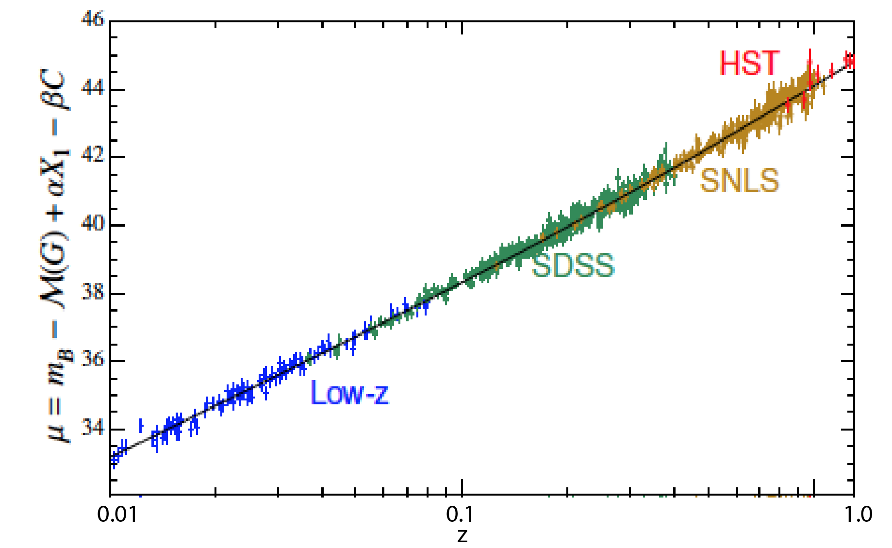
Figure from Betoule et al. (2014), Astronomy and Astrophysics 568, A22.
The setup cell loaded the table as far_supernovae. Look at it before you use it:
print(len(far_supernovae), "rows, nearest first; the first five:")
far_supernovae.head()
31 rows, nearest first; the first five:
| z | VCMB | D(Mpc) | |
|---|---|---|---|
| 0 | 0.010 | 2982.935699 | 38.974217 |
| 1 | 0.012 | 3575.925975 | 59.676137 |
| 2 | 0.014 | 4167.717590 | 58.671628 |
| 3 | 0.016 | 4758.310727 | 66.636687 |
| 4 | 0.019 | 5641.953747 | 82.925710 |
✏️ Your turn 9
Does the line from class still work twenty times farther away?
Why: the class line was fitted to supernovae between 56.0 and 467.0 Mpc. Using a line outside the range of its data is extrapolation. This part tests it on real measurements.
class_line_speed: askorigin_model, the class line through the origin from Your turn 7, what speed it gives at each of the far distances.- The figure: three things on one figure: the far supernovae, the supernovae from class as smaller red dots, and the line.
line_fastest,table_fastestandtimes_too_fast: the largest speed the line gives and the largest speed in the table, which both belong to the farthest row, and the first divided by the second.
So: at the farthest supernova, how many times too fast is the line?
Use these names, because the self-check looks for them: class_line_speed and
times_too_fast.
class_line_speed = origin_model.predict(far_supernovae[["D(Mpc)"]])

plt.figure(figsize=(7, 4))
plt.scatter(far_supernovae["D(Mpc)"], far_supernovae["VCMB"], color="tab:blue", label="far supernovae")
plt.scatter(supernovae["D(Mpc)"], supernovae["VCMB"], color="tab:red", s=8, label="supernovae from class")
plt.plot(far_supernovae["D(Mpc)"], class_line_speed, color="black", label="the line fitted in class")
plt.xlabel("distance (Mpc)")
plt.ylabel("speed away from us (km/s)")
plt.legend()
plt.title(f"The line from class, extended to far supernovae (n = {len(far_supernovae)} rows)")
plt.show()

line_fastest = class_line_speed.max()
table_fastest = far_supernovae["VCMB"].max()
times_too_fast = line_fastest / table_fastest
print("at the farthest supernova the line gives", round(line_fastest), "km/s; the table has", round(table_fastest), "km/s")
print("the line is", round(times_too_fast, 1), "times too fast")

at the farthest supernova the line gives 651016 km/s; the table has 204469 km/s
the line is 3.2 times too fast
# Self-check: run this after your answer. You do not need to read it — it only says whether something is off.
assert len(class_line_speed) == len(far_supernovae) and abs(class_line_speed - origin_model.predict(far_supernovae[["D(Mpc)"]])).max() < 1000, "class_line_speed is the class line's prediction at the far distances: origin_model.predict on far_supernovae[[\"D(Mpc)\"]]"
assert abs(times_too_fast - class_line_speed.max() / far_supernovae["VCMB"].max()) < 0.06 and line_fastest > table_fastest, "times_too_fast is line_fastest, the largest speed the line gives, divided by table_fastest, the largest speed in the table"
print(f"✓ Your turn 9 — at the farthest supernova the line gives {round(class_line_speed.max())} km/s, {round(times_too_fast, 1)} times the speed in the table")
✓ Your turn 9 — at the farthest supernova the line gives 651016 km/s, 3.2 times the speed in the table
What the numbers mean. Inside the range of the class data, the crowded lower-left corner of the figure, the far supernovae lie within about 15 percent of the line, 12 of 14 a little below it. Beyond that range they fall farther and farther below, and at the farthest one the line gives 651,016 km/s where the table has 204,469: 3.2 times too fast, and more than twice the speed of light, which nothing can reach. The line was fitted to supernovae between 56.0 and 467.0 Mpc, and there it fits well. Nothing in the fit said it would hold 20 times farther out, and it does not. A fitted line describes the range of its data; using it far outside that range is extrapolation, and it is a guess. How large the miss is depends on how speed and distance are worked out that far away. With the speed worked out from the redshift and the distance from the brightness, as in this table, a straight line fails. The class result is not wrong: it is a result about the nearby universe.
✏️ Your turn 10
Would a new straight line through the far supernovae fix it?
Why: the class line failed far away. Perhaps the far data only need a line of their own. R² and the residual plot, the two tools of Your turn 6, can tell.
far_model: a fresh line fitted tofar_supernovaeitself. Let the fit choose its intercept too (a free line, as in Your turn 5), to give the line every chance.new_line_speedandfar_residuals: the new line's speed at each far distance, and the residuals.- The figure: two panels side by side, with the panels and labels given: the far supernovae with their line, and the residuals against distance.
far_r_squared,far_slopeandfar_age: the line's R², its slope, and the age that slope would give, fromage_of_universe.
So: R² is the share of the flat line's miss that the line removes. Do the residuals agree that a straight line describes these data?
Use these names, because the self-check looks for them: far_model, new_line_speed,
far_residuals, far_r_squared, far_slope and far_age.
far_model = LinearRegression().fit(far_supernovae[["D(Mpc)"]], far_supernovae["VCMB"])
new_line_speed = far_model.predict(far_supernovae[["D(Mpc)"]])
far_residuals = far_supernovae["VCMB"] - new_line_speed

plt.figure(figsize=(9, 4))
plt.subplot(1, 2, 1)
plt.scatter(far_supernovae["D(Mpc)"], far_supernovae["VCMB"], color="tab:blue")
plt.plot(far_supernovae["D(Mpc)"], new_line_speed, color="black")
plt.xlabel("distance (Mpc)")
plt.ylabel("speed away from us (km/s)")
plt.title(f"A line through the far supernovae (n = {len(far_supernovae)} rows)")

plt.subplot(1, 2, 2)
plt.scatter(far_supernovae["D(Mpc)"], far_residuals, color="tab:blue")
plt.axhline(0, color="black")
plt.xlabel("distance (Mpc)")
plt.ylabel("residual (km/s)")
plt.title("What that line misses")
plt.tight_layout()  # keeps the two panels from overlapping
plt.show()

far_r_squared = far_model.score(far_supernovae[["D(Mpc)"]], far_supernovae["VCMB"])
far_slope = far_model.coef_[0]
far_age = age_of_universe(far_slope)
print("R²:", round(far_r_squared, 3))
print("slope:", round(far_slope, 1), "km/s per Mpc, which would make the universe", round(far_age, 1), "billion years old (class: 13.84)")

R²: 0.921
slope: 24.5 km/s per Mpc, which would make the universe 40.0 billion years old (class: 13.84)
# Self-check: run this after your answer. You do not need to read it — it only says whether something is off.
assert 24 < far_model.coef_[0] < 25 and far_model.intercept_ != 0, "far_model is a new FREE line fitted to far_supernovae: distance as x and speed as y"
assert len(new_line_speed) == len(far_supernovae) and abs(new_line_speed - far_model.predict(far_supernovae[["D(Mpc)"]])).max() < 1, "new_line_speed is far_model.predict on the far distances, as a one-column table"
assert (far_residuals > 0).sum() == 14 and abs(far_residuals.max() - 28241) < 50, "far_residuals is the real speed of far_supernovae minus the NEW line's speed: far_model.predict, not the line from class"
assert abs(far_r_squared - far_model.score(far_supernovae[["D(Mpc)"]], far_supernovae["VCMB"])) < 0.005, "far_r_squared is far_model.score on the same two things the fit was given"
assert isinstance(far_slope, float) and abs(far_slope - far_model.coef_[0]) < 0.06, "far_slope is the new line's slope: far_model.coef_[0]"
assert abs(far_age - age_of_universe(far_model.coef_[0])) < 0.3 and 39 < far_age < 41, "far_age is age_of_universe called on far_slope. If the call is right, look again at your function in Your turn 7"
print(f"✓ Your turn 10 — R² is {round(far_r_squared, 3)}, and a slope of {round(far_slope, 1)} km/s per Mpc would mean {round(far_age, 1)} billion years")
✓ Your turn 10 — R² is 0.921, and a slope of 24.5 km/s per Mpc would mean 40.0 billion years
What the numbers mean. The new line has an R² of 0.921, which sounds like a good fit, and a slope of 24.5 km/s per Mpc, which would make the universe 40.0 billion years old. The residuals show what R² hides, as the bottom row of the correlation gallery warned: the nearest 15 rows all sit below the line (they overlap at the left edge of the panel), the next 14 sit above it, and the last 2 below again. That is an arch, not noise. The data curve, so no straight line can describe them, and a slope taken from one means little. The next part fits the curve, the way astronomers do.
A curve is one more column. The residuals of Your turn 10 arch, so the far supernovae want a curve, not a line. A line is $y = a\,x + b$: one column, $x$, with one slope. Give the fit a second column and it finds a second slope for it:
$$y = a_1\,x + a_2\,x_2 + b$$
Now make that second column the first one squared, $x_2 = x^2$. The rule becomes
$y = a_1\,x + a_2\,x^2 + b$, and that is a curve: it bends upward if $a_2$ is positive and
bends over if $a_2$ is negative. To scikit-learn nothing has changed. It is still choosing
numbers to make the RMSE as small as it can, by the same least squares, and it does not care
that one column was made from another. The fit is the same call with two columns inside the
double brackets, [["D(Mpc)", "d2"]]; coef_ then holds two numbers, $a_1$ and $a_2$, one per
column, and intercept_ is still $b$.
So the only new line is the one that makes the squared column. A table gets a new column when
you assign to a name it does not have yet, with a whole old column on the right, as the
earthquake week made region out of place:
table["new"] = table["old"] ** 2
Here the table is far_supernovae, the old column is D(Mpc) and the new one is d2.
✏️ Your turn 11
Does a curve fix it, and what does the curve mean?
Why: Your turn 10 showed that a straight line is the wrong shape for the far supernovae. A curve through the same data, on the same axes, tests whether one more term is enough, and the residual plot says whether any pattern is left.
far_supernovae["d2"]: the new column, the distance squared, made as the cell above shows: theD(Mpc)column, squared, assigned to the named2.far_curve: a free fit, as in Your turn 10, but with two columns,[["D(Mpc)", "d2"]].curve_speedandcurve_residuals: the curve's speed at each far distance, frompredictwith the same two columns, and the real speed minus it.curve_rmseandcurve_r_squared: the RMSE of the residuals, and R² fromfar_curve.score, with the same two things the fit was given.- The figure is given: the data with the line of Your turn 10 and your curve, and the residuals
of both. It uses
new_line_speed,far_residualsandfar_r_squaredfrom Your turn 10, so that part must be done first.
So: how much of the miss does the curve remove, and is the residual plot now patternless?
Use these names, because the self-check looks for them: far_curve, curve_speed,
curve_residuals, curve_rmse and curve_r_squared.
far_supernovae["d2"] = far_supernovae["D(Mpc)"] ** 2
far_curve = LinearRegression().fit(far_supernovae[["D(Mpc)", "d2"]], far_supernovae["VCMB"])
curve_speed = far_curve.predict(far_supernovae[["D(Mpc)", "d2"]])
curve_residuals = far_supernovae["VCMB"] - curve_speed
curve_rmse = ((curve_residuals ** 2).mean()) ** 0.5
curve_r_squared = far_curve.score(far_supernovae[["D(Mpc)", "d2"]], far_supernovae["VCMB"])

plt.figure(figsize=(10, 4))
plt.subplot(1, 2, 1)
plt.scatter(far_supernovae["D(Mpc)"], far_supernovae["VCMB"], color="tab:blue", label="far supernovae")
plt.plot(far_supernovae["D(Mpc)"], new_line_speed, color="black", label="the line of Your turn 10")
plt.plot(far_supernovae["D(Mpc)"], curve_speed, color="red", label="your curve")
plt.xlabel("distance (Mpc)")
plt.ylabel("speed away from us (km/s)")
plt.legend(fontsize=8)
plt.title(f"A line and a curve through the far supernovae (n = {len(far_supernovae)})")
plt.subplot(1, 2, 2)
plt.scatter(far_supernovae["D(Mpc)"], far_residuals, color="black", label="the line's residuals")
plt.scatter(far_supernovae["D(Mpc)"], curve_residuals, color="red", label="the curve's residuals")
plt.axhline(0, color="gray")
plt.xlabel("distance (Mpc)")
plt.ylabel("residual (km/s)")
plt.legend(fontsize=8)
plt.title("What each one misses")
plt.tight_layout()
plt.show()

print("the line:  RMSE", round(((far_residuals ** 2).mean()) ** 0.5), "km/s   R²", round(far_r_squared, 3))
print("the curve: RMSE", round(curve_rmse), "km/s   R²", round(curve_r_squared, 3))
print("the curve's three numbers: a1 =", round(far_curve.coef_[0], 1), " a2 =", round(far_curve.coef_[1], 5), " b =", round(far_curve.intercept_))

the line:  RMSE 17140 km/s   R² 0.921
the curve: RMSE 4971 km/s   R² 0.993
the curve's three numbers: a1 = 45.8  a2 = -0.00276  b = 5795
# Self-check: run this after your answer. You do not need to read it — it only says whether something is off.
assert "d2" in far_supernovae.columns and abs(far_supernovae["d2"].max() - far_supernovae["D(Mpc)"].max() ** 2) < 1, "d2 is the D(Mpc) column squared, added to far_supernovae"
assert len(far_curve.coef_) == 2 and far_curve.intercept_ != 0, "far_curve is a FREE fit with two columns: far_supernovae[[\"D(Mpc)\", \"d2\"]], then its speed"
assert len(curve_speed) == len(far_supernovae) and abs(curve_speed - far_curve.predict(far_supernovae[["D(Mpc)", "d2"]])).max() < 1, "curve_speed is far_curve.predict on the same two columns"
assert abs(curve_rmse - 4971) < 5, "curve_rmse is the RMSE of the real speed minus curve_speed: squared, averaged, ** 0.5"
assert abs(curve_r_squared - 0.993) < 0.002, "curve_r_squared is far_curve.score on the two columns and the speed"
print(f"✓ Your turn 11 — the curve misses by {round(curve_rmse):,} km/s, against the line's {round(((far_residuals ** 2).mean()) ** 0.5):,}, with R² {round(curve_r_squared, 3)}")
✓ Your turn 11 — the curve misses by 4,971 km/s, against the line's 17,140, with R² 0.993
What the numbers mean. The curve is much better and still not right. Its RMSE is 4,971 km/s against the line's 17,140, and R² rises from 0.921 to 0.993. But the residual plot still has a shape, 12 below, then 14 above, then below again: a curve with one bend is not quite the shape of these data either.
And the curve's numbers have no physical meaning. Its $a_2$ is negative, so the curve bends
over and would start to fall beyond about 8,300 Mpc, as if the farthest galaxies
slowed down. That is a property of the columns, not of the universe. The speed in VCMB was
worked out from the redshift by a formula that can never exceed the speed of light, while the
distance keeps growing, so any curve through these points must flatten, in a universe that is
speeding up or in one that is slowing down. The bend cannot tell the two apart. Astronomers fit
distance against the redshift itself, the thing the spectrograph measures, with a $z^2$ term
like your d2, and there the size of the bend measures whether the expansion is slowing down
or speeding up today. In 1998 two teams fitted supernovae like these and found it speeding up,
the discovery that won the 2011 Nobel prize; the cause was named dark energy. It is also why the
published age is so close to 1/H₀: with gravity alone the universe would be only two thirds of
that, about 9.2 billion years old, and the speeding-up since has
nearly cancelled the early slowing, as section 4 said.