When will CO2 pass 450 ppm?
EPS 88 · PyEarth. Open your own copy on DataHub: click here.
Every month since March 1958, an observatory high on Mauna Loa, a volcano in Hawaii, has measured how much carbon dioxide (CO2) is in the air. It is the longest record of its kind, and its yearly average has gone up every single year. It now stands near 430 parts per million. When will it pass 450?
To answer, you need a curve that follows the record, and a fair way to tell a curve that has learned the pattern from one that has only memorised the past. Today you fit four curves, choose between them on years they never saw, test the winner once on the most recent years, and read its forecast. Then you see how much that forecast depends on the choice. At home you repeat the method at two more stations, one in the Arctic and one at the South Pole.
Every place you write something opens with a pencil icon and the words Your turn, and is
followed by a cell that already has the shape of the answer written in, with ... wherever your
code goes. Replace every ..., run every cell so your answers and figures are
saved in the file, then download this notebook itself — the .ipynb file — and upload it
to Gradescope. Not a PDF: the marking reads your notebook, and a PDF cannot be read.
In JupyterLab: File ▸ Download, or right-click the file in the left-hand panel and choose
Download.
Two habits from the first minute. A cell runs when you press Shift+Enter, and the notebook remembers everything it has already run — so when something breaks and you cannot see why, Kernel → Restart Kernel and Run All Cells throws the memory away and rebuilds it from the top. That is never the wrong thing to do.
What you'll be able to do
The science. Describe the two patterns in the CO2 record, the long rise and the yearly breath; say when the yearly average reaches 450 ppm by the curve the data choose; and explain why that date is less certain than the fit makes it look.
The code. A new column made from an old one (a square, a sine, a cosine) · fitting on
training months, choosing on validation months, testing once · a loop that compares four models ·
np.sin, np.cos and np.pi.
Thirteen places where you write something: nine in class, four at home. Each is headed
Your turn, and the cell under it has the shape of the answer written in, with ... wherever
your code goes and a comment beside each one saying what goes there.
The four questions of the class:
- What does the CO2 record show?
- How do we choose a curve we can trust on years it has not seen?
- When will CO2 pass 450 ppm?
- How far can we trust that answer?
Setup
Run the next cell once. It reads NOAA's Mauna Loa file (live if the network is up, the copy stored with the course if not) and the two stations for the homework, which are stored with the course. Then it adds two columns to each table:
time: the middle of each month, written as a year with decimals (March 1958 is 1958.21);decades: the time since 1958, counted in decades (2026 is 6.8 decades).
Counting in decades keeps the numbers small. Later you will square this column and take higher powers of it; counted in years, the fourth power of 2026's value would be about 20 million, far too large for the fit to handle well.
(The numbers quoted in this notebook come from the stored copy; if your notebook read NOAA's live file, a few may differ in their last digit.)
import numpy as np
from sklearn.linear_model import LinearRegression
import pandas as pd
import matplotlib.pyplot as plt

# house style, set once, so every plot cell below holds only what matters
plt.rcParams.update({"figure.dpi": 110,
                     "axes.grid": True, "grid.alpha": 0.3, "axes.axisbelow": True})

CACHE = "https://raw.githubusercontent.com/AI4EPS/EPS88_PyEarth/main/data"

def load():
    """NOAA's Mauna Loa monthly CO2 file: live if the network is up, the copy stored with the course if not"""
    # Ask the live archive first. If it is down, or you are offline, read the copy stored with
    # the course instead, so the notebook still runs.
    try:
        return pd.read_csv("https://gml.noaa.gov/webdata/ccgg/trends/co2/co2_mm_mlo.csv", comment="#")
    except Exception as e:
        print("live source unreachable, using the cached copy:", type(e).__name__)
        return pd.read_csv(CACHE + "/" + "week09_co2_mm_mlo.csv")

# mlo, brw and spo are NOAA's codes for the three stations: Mauna Loa, Barrow and the South Pole.
mlo = load()
# Keep the months up to July 2026, the last month in the stored copy, so every notebook gets the same numbers.
mlo = mlo[mlo["decimal date"] < 2026.6]     # NOAA's own time column: July 2026 is 2026.54
mlo["co2"] = mlo["average"]      # each month's average CO2, in parts per million (ppm)
# After Mauna Loa erupted, the months from December 2022 to early July 2023 were measured on
# Maunakea, about 21 miles north. NOAA fills the few months with no measurement by interpolation.

# For the homework: Barrow, Alaska (71° N) and the South Pole (90° S), stored with the course.
# NOAA marks a month with no measurement -999.99; those few months are already removed.
brw = pd.read_csv(CACHE + "/week07_co2_brw.csv")
spo = pd.read_csv(CACHE + "/week07_co2_spo.csv")

for table in [mlo, brw, spo]:
    table["time"] = table["year"] + (table["month"] - 0.5) / 12    # the middle of each month, as a year
    table["decades"] = (table["time"] - 1958) / 10                  # time since 1958, in decades

print("Mauna Loa:", len(mlo), "months, from", mlo["year"].min(), "to", mlo["year"].max())
print("Barrow:", len(brw), "months.  South Pole:", len(spo), "months.")
1. What does the CO2 record show?
CO2 is counted in parts per million. A reading of 430 ppm means that in every million molecules of air, 430 are carbon dioxide. That is a small share, but CO2 lets sunlight in and holds back some of the heat the ground gives off. It is one of the gases behind the greenhouse effect from the liquid-water week: the difference between the temperature a world would have with no air and the temperature it actually has.
Where the numbers come from. Charles David Keeling began measuring CO2 on Mauna Loa in March 1958. The observatory sits 3,397 m up the volcano's side, far from cities and forests, so the air it samples has mixed over a wide area; one station there tells you about much of the planet.
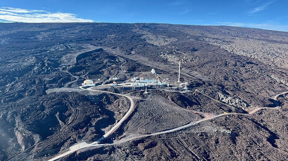
The Mauna Loa Observatory on the volcano's bare lava slope. Photo: Brian Vasel, NOAA (public domain), via Wikimedia Commons.
Why it rises. Burning coal, oil and gas, and clearing forests, release CO2. About half of what people emit stays in the air (48 percent over 2014–2023, by the Global Carbon Budget 2024); the oceans and the land take up the rest. Carbon is always moving between the air, plants, soils and the ocean; burning fossil fuels adds a flow that had no return path on human time scales.
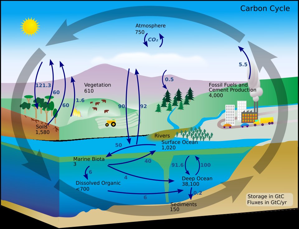
The carbon cycle: where carbon is stored (black numbers, billions of tonnes) and how fast it moves (arrows, billions of tonnes a year). The numbers are from the 1990s; today the air holds more, and fossil fuels add more each year. The shape of the cycle is what matters here. Diagram: NASA Earth Observatory, redrawn by Kevin Saff and FischX (public domain), via Wikimedia Commons.
How unusual is today's level? Bubbles of old air trapped in the Antarctic ice sheet record CO2 long before anyone measured it. Through the ice ages of the last 800,000 years it swung from below 200 ppm in the coldest times to about 300 in the warmest, and it did not go above 300 until the industrial age:
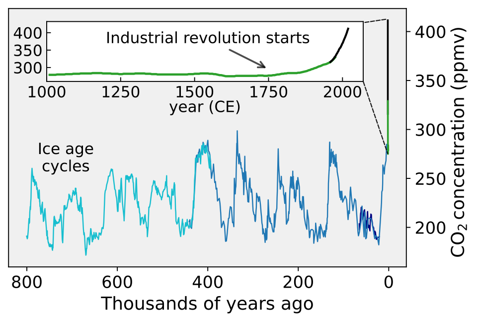
CO2 over the last 800,000 years from ice cores, with the last thousand years enlarged; the steep black end is the age of measurements like Mauna Loa's. Figure: Femke Nijsse (CC BY-SA 3.0), via Wikimedia Commons.
mlo[["year", "month", "co2", "time", "decades"]].head()
✏️ Your turn 1
What does the record look like?
Why: before fitting any curve, look at the data. What you see decides which curves are worth trying.
- The figure. Draw the monthly CO2 against time as a line, with a label and units on each axis.
highestandlowest: the largest and the smallest value of theco2column.
Use these names, because the self-check looks for them: highest and lowest.
# ← your answer here: replace every ... with code
plt.figure(figsize=(8, 4))
plt.plot(..., ...)  # time across, CO2 up
plt.xlabel(...)     # what runs across, with its units
plt.ylabel(...)     # what runs up, with its units
plt.title(f"Mauna Loa, every month ({len(mlo)} months)")
plt.show()

highest = ...  # the largest monthly CO2
lowest = ...   # the smallest monthly CO2
print("CO2 has ranged from", lowest, "to", highest, "ppm")
# Self-check: run this after your answer. You do not need to read it — it only says whether something is off.
assert highest == 432.34 and lowest == 312.42, "highest and lowest are the largest and smallest values of the co2 column"
print(f"✓ Your turn 1 — CO2 has ranged from {lowest} to {highest} ppm")
Two patterns. The first is the long rise, and it is not a straight line: the curve gets steeper as the years go on. The second is a ripple of teeth, one tooth a year. Three years drawn close up show what the teeth are:
plt.figure(figsize=(8, 4))
for year in [2021, 2022, 2023]:
    one_year = mlo[mlo["year"] == year]
    plt.plot(one_year["month"], one_year["co2"], marker="o", label=str(year))
plt.xlabel("month (1 = January)")
plt.ylabel("CO2 (ppm)")
plt.title("Three years close up, one line per year")
plt.legend()
plt.show()
Each year CO2 climbs to a high in May and falls to a low in September or October, and each high sits above the last. The yearly fall comes from plants. Most of the world's land that has a winter is in the northern half of the planet: forests and grasslands that green up together in spring and summer, taking CO2 out of the air, and lose their leaves together in autumn and winter, when decay gives it back. Mauna Loa, at 19.5° N, breathes with the north.
So a curve that follows this record needs two things: a rise that gets steeper, and a ripple that repeats every twelve months. The next section builds one piece at a time, and asks how to tell whether each piece helps.
2. How do we choose a curve we can trust on years it has not seen?
A curve that fits the past is not yet a curve to trust about the future. A flexible enough curve can pass close to every month in the record and still be wrong about next year, because it has learned the record's accidents along with its pattern. The fair test is to hide some years from the curve and see how well it does on them. In short: hide some data from yourself, then check.
Three sets, as for an exam. Think of studying:
- the homework problems are what you learn from;
- a practice exam tells you whether your way of studying works, and you may change your way of studying after seeing it;
- the final exam is taken once, at the end. If you took it again and again, changing your answers each time, it would stop measuring what you know.
A model gets the same three sets of data, here three spans of years:
- training months, 1958–2000: each curve learns from these;
- validation months, 2001–2010: years held back to choose between models. Once they have chosen, they are no longer a fair test.
- test months, 2011 onward: years nobody looks at until the end, checked once, on the model already chosen.
Why years in order, and not a random third of the months? Because a forecast is about the future. Months picked at random would sit between training months, where any smooth curve does well, and the test would say nothing about years to come. That would be leakage: any route by which information about the data you are scoring on reaches the model before you score it.
✏️ Your turn 2
Which months does each set hold?
Why: every fit and every score below uses these three sets. Each is a mask on the year
column, written with the table skills of the tables week.
training: True for the months up to the end of 2000.validation: True for the months from 2001 to 2010, both years included.test: True for the months from 2011 on.
Use these names, because the self-check looks for them: training, validation and test.
# ← your answer here: replace every ... with code
training = ...              # the months up to the end of 2000
validation = (...) & (...)  # the months from 2001 to 2010, both included
test = ...                  # the months from 2011 on
print("months:", training.sum(), "training,", validation.sum(), "validation,", test.sum(), "test")
# Self-check: run this after your answer. You do not need to read it — it only says whether something is off.
assert training.sum() == 514 and validation.sum() == 120 and test.sum() == 187, "the three sets are the months up to 2000, 2001 to 2010, and 2011 on"
assert not (training & validation).any() and not (validation & test).any(), "no month may be in two sets"
print(f"✓ Your turn 2 — {training.sum()} training, {validation.sum()} validation and {test.sum()} test months")
plt.figure(figsize=(8, 4))
plt.plot(mlo[training]["time"], mlo[training]["co2"], label="training: the curves learn from these")
plt.plot(mlo[validation]["time"], mlo[validation]["co2"], label="validation: we choose with these")
plt.plot(mlo[test]["time"], mlo[test]["co2"], label="test: checked once, at the end")
plt.xlabel("year")
plt.ylabel("CO2 (ppm)")
plt.title("The record in three parts")
plt.legend()
plt.show()
How a curve's miss is measured. As in the age-of-the-universe week: a residual is the data minus what the curve says, one per month, and the root mean squared error (RMSE) sums them up. Square every residual, average the squares, take the square root. The result is a typical miss, in ppm. Here it is always worked out on the validation months, the years the curve did not learn from.
✏️ Your turn 3
How badly does a straight line miss the validation years?
Why: the straight line is the simplest curve, and the one to beat. It is the age-of-the-universe line, with time across instead of distance.
line: a straight line fitted to the training months:decadesacross (as a one-column table),co2up.residuals: the validation months' CO2 minus what the line says for them.line_validation_rmse: the RMSE of those residuals.- The figure: the line drawn over the whole record.
Use these names, because the self-check looks for them: line and line_validation_rmse.
# ← your answer here: replace every ... with code
line = LinearRegression().fit(..., ...)  # the training months: decades as a one-column table, then co2
residuals = ... - ...                    # the validation months' co2, minus what the line says for those months
line_validation_rmse = ...               # square the residuals, average, then take the square root
print("the straight line misses the validation months by", round(line_validation_rmse, 2), "ppm")

plt.figure(figsize=(8, 4))
plt.plot(mlo["time"], mlo["co2"], color="0.7", label="data")
plt.plot(..., ..., label="straight line, fitted to 1958-2000")  # time across, the line's CO2 for every month up
plt.xlabel("year")
plt.ylabel("CO2 (ppm)")
plt.title("A straight line")
plt.legend()
plt.show()
# Self-check: run this after your answer. You do not need to read it — it only says whether something is off.
assert abs(line_validation_rmse - 7.18) < 0.01, "fit on the training months, then measure the miss on the validation months"
print(f"✓ Your turn 3 — the straight line misses the validation months by {line_validation_rmse:.2f} ppm")
The line misses by 7.18 ppm, and the figure shows why: the record curves upward away from it: from 2001 on, almost every month lies above the line.
A new column lets a line-fitting method draw a curve. In the age-of-the-universe homework you
gave the fit a second column, the distance squared. The fit finds one number for each column it
is given, so with decades and decades squared it fits
$$\text{CO2} = a \times \text{decades} + c \times \text{decades}^2 + b$$
The squared term is small near 1958 and grows fast later, which is exactly the shape of a rise that gets steeper. Nothing else changes: the same fit, the same masks, the same RMSE.
✏️ Your turn 4
Does a squared column help on the validation years?
Why: the record bends upward; a squared column is the simplest way to let the curve bend.
mlo["decades2"]: a new column, thedecadescolumn squared.squared: the curve fitted to the training months with bothdecadesanddecades2.squared_validation_rmse: its miss on the validation months.- The figure: the curve over the whole record.
Use these names, because the self-check looks for them: squared and squared_validation_rmse.
# ← your answer here: replace every ... with code
mlo["decades2"] = ...                       # the decades column, squared
squared = LinearRegression().fit(..., ...)  # the training months: the two columns, then co2
residuals = ... - ...                       # the validation months' co2, minus what the curve says
squared_validation_rmse = ...               # the typical miss, as before
print("the squared curve misses the validation months by", round(squared_validation_rmse, 2), "ppm")

plt.figure(figsize=(8, 4))
plt.plot(mlo["time"], mlo["co2"], color="0.7", label="data")
plt.plot(..., ..., label="squared curve, fitted to 1958-2000")  # time across, the curve's CO2 for every month
plt.xlabel("year")
plt.ylabel("CO2 (ppm)")
plt.title("A curve with a squared column")
plt.legend()
plt.show()
# Self-check: run this after your answer. You do not need to read it — it only says whether something is off.
assert "decades2" in mlo.columns and abs(mlo["decades2"].max() - mlo["decades"].max() ** 2) < 1e-6, "decades2 is the decades column squared"
assert abs(squared_validation_rmse - 2.2) < 0.01, "fit decades and decades2 on the training months, measure on the validation months"
print(f"✓ Your turn 4 — the squared curve misses by {squared_validation_rmse:.2f} ppm, against {line_validation_rmse:.2f} for the line")
From 7.18 ppm to 2.2: the bend was most of what the line missed. What is left is mainly the teeth, which neither curve can draw.
A wave repeats every twelve months, and two columns can draw one. Turn each month into an angle around a circle, one full turn a year: $\text{angle} = 2\pi \times (\text{month} - 0.5) / 12$. (A full turn is $2\pi$; the $-0.5$ puts each month at its middle.) The sine of that angle rises and falls once a year, and so does the cosine, a quarter of a year later. Drawn over twelve months:
month_numbers = np.arange(1, 13)
month_angle = 2 * np.pi * (month_numbers - 0.5) / 12

plt.figure(figsize=(7, 3.5))
plt.plot(month_numbers, np.sin(month_angle), marker="o", label="sine of the month's angle")
plt.plot(month_numbers, np.cos(month_angle), marker="o", label="cosine of the month's angle")
plt.axhline(0, color="0.5", lw=0.8)
plt.ylim(-1.2, 1.7)     # room at the top for the legend
plt.xlabel("month (1 = January)")
plt.ylabel("value")
plt.title("Two waves, each one cycle a year")
plt.legend(loc="upper center", ncol=2)
plt.show()
The sine is highest in March and April and lowest in September and October; the cosine is highest in December and January and lowest in June and July. Give the fit both, and it chooses how much of each, which lets the mixed wave peak in any month and be any size. Each is a seasonal column: a column that rises and falls once a year, so the fitted curve can rise and fall with the seasons. The curve is now
$$\text{CO2} = a \times \text{decades} + c \times \text{decades}^2 + s \times \sin(\text{angle}) + k \times \cos(\text{angle}) + b$$
✏️ Your turn 5
Do two seasonal columns help on the validation years?
Why: the teeth are what the squared curve still misses. Two waves, one fit, should draw them.
angle: each month's angle, by the formula above, from themonthcolumn.mlo["sin_month"]andmlo["cos_month"]: two new columns, the sine and the cosine of each month's angle.seasonal: the curve fitted to the training months withdecades,decades2,sin_monthandcos_month.seasonal_validation_rmse: its miss on the validation months.
Use these names, because the self-check looks for them: seasonal and
seasonal_validation_rmse.
# ← your answer here: replace every ... with code
angle = ...             # each month's angle: a full turn, 2 pi, times the month's middle as a share of the year
mlo["sin_month"] = ...  # the sine of each month's angle
mlo["cos_month"] = ...  # the cosine of each month's angle

columns = ["decades", "decades2", "sin_month", "cos_month"]
seasonal = LinearRegression().fit(..., ...)  # the training months: these four columns, then co2
residuals = ... - ...                        # the validation months' co2, minus what the curve says
seasonal_validation_rmse = ...               # the typical miss
print("with the seasons, the curve misses the validation months by", round(seasonal_validation_rmse, 2), "ppm")

validation_decade = mlo[validation]
plt.figure(figsize=(8, 4))
plt.plot(validation_decade["time"], validation_decade["co2"], color="0.6", marker=".", label="data")
plt.plot(..., ..., label="squared curve with seasons, fitted to 1958-2000")  # the validation months' time, and the curve's CO2 for them
plt.xlabel("year")
plt.ylabel("CO2 (ppm)")
plt.title(f"The validation months, close up ({len(validation_decade)} months)")
plt.legend()
plt.show()
# Self-check: run this after your answer. You do not need to read it — it only says whether something is off.
assert abs(mlo["sin_month"].max() - 0.9659) < 0.001 and abs(mlo["cos_month"].min() + 0.9659) < 0.001, "sin_month and cos_month are np.sin and np.cos of angle"
assert abs(seasonal_validation_rmse - 0.77) < 0.01, "fit the four columns on the training months, measure on the validation months"
print(f"✓ Your turn 5 — with the seasons the miss falls to {seasonal_validation_rmse:.2f} ppm")
More columns always fit the training months better. They do not always fit new months better. The squared curve with seasons misses the validation decade by only 0.77 ppm. Why stop there? A cubed column, or a fourth power, would bend the curve more freely and fit 1958–2000 even more closely. The risk has a name, overfitting: a curve that memorises the data you gave it fails on the data you did not. The highest power in a curve is its degree: the degree of a polynomial is how many bends it is allowed: degree 1 is a straight line, degree 2 bends once.
The way to find out is to try each degree and score it on the validation months. The figure that shows the answer is a validation curve: plot the miss on the training years and on the held-back years against how flexible the curve is; the flexibility worth choosing is where the held-back miss is lowest.
✏️ Your turn 6
Which of four curves should we trust?
Why: this is the choice itself. Each candidate keeps the two seasonal columns and adds one more
power of decades. The loop fits each one to the training months and scores it twice: on the
training months it learned from, and on the validation months it did not.
- The new columns, the candidates and their names are given.
- Inside the loop, for each list of columns: fit to the training months, then append the
training RMSE to
training_rmsesand the validation RMSE tovalidation_rmses. best: the name of the candidate with the smallest validation RMSE, found withnp.argmin, as in the age-of-the-universe week.- The figure: both lists of RMSE, one point per candidate.
Use these names, because the self-check looks for them: training_rmses, validation_rmses
and best.
# ← your answer here: replace every ... with code
mlo["decades3"] = mlo["decades"] ** 3
mlo["decades4"] = mlo["decades"] ** 4
season = ["sin_month", "cos_month"]
candidates = [["decades"] + season,
              ["decades", "decades2"] + season,
              ["decades", "decades2", "decades3"] + season,
              ["decades", "decades2", "decades3", "decades4"] + season]
names = ["line", "squared", "cubed", "fourth power"]

training_rmses = []
validation_rmses = []
for columns in candidates:
    model = LinearRegression().fit(..., ...)  # this candidate's columns, on the training months
    residuals = ... - ...                     # the training months' co2, minus what the model says
    training_rmses.append(...)                # the typical training miss
    residuals = ... - ...                     # the validation months' co2, minus what the model says
    validation_rmses.append(...)              # the typical validation miss

best = ...  # the name at the position of the smallest validation RMSE
for i in range(4):
    print(names[i], ": training", round(training_rmses[i], 2), "ppm,  validation", round(validation_rmses[i], 2), "ppm")
print("the validation months choose:", best)

plt.figure(figsize=(7, 4))
plt.plot(names, ..., marker="o", label="training months (1958-2000)")    # the training RMSEs
plt.plot(names, ..., marker="o", label="validation months (2001-2010)")  # the validation RMSEs
plt.xlabel("candidate curve (each with the two seasonal columns)")
plt.ylabel("RMSE (ppm)")
plt.title("Four curves, scored twice")
plt.legend()
plt.show()
# Self-check: run this after your answer. You do not need to read it — it only says whether something is off.
assert len(training_rmses) == 4 and len(validation_rmses) == 4, "one training and one validation RMSE per candidate"
assert [round(x, 2) for x in validation_rmses] == [6.85, 0.77, 4.51, 3.31], "score each candidate on the validation months, after fitting it on the training months"
assert best == "squared", "best is the name with the smallest validation RMSE"
print(f"✓ Your turn 6 — the validation months choose the {best} curve")
plt.figure(figsize=(8, 4))
shown = mlo["year"] <= 2010
plt.plot(mlo[shown]["time"], mlo[shown]["co2"], color="0.7", label="data")
for i in range(4):
    model = LinearRegression().fit(mlo[training][candidates[i]], mlo[training]["co2"])
    plt.plot(mlo[shown]["time"], model.predict(mlo[shown][candidates[i]]), label=names[i])
plt.axvline(2001, color="black", lw=0.8)
plt.xlim(1985, 2011)
plt.ylim(340, 400)
plt.xlabel("year (the black line: training months to its left, validation months to its right)")
plt.ylabel("CO2 (ppm)")
plt.title("The four curves, fitted to 1958-2000, carried into 2001-2010")
plt.legend()
plt.show()
The two lines tell different stories. On the training months every extra power helps, or at least does no harm: 1.92, 0.97, 0.82 and 0.82 ppm. On the validation months the squared curve wins clearly, 0.77 ppm, and the cubed and fourth-power curves are four to six times worse (4.51 and 3.31). The extra powers let the curve follow small bends in the 1958–2000 record, which buys almost nothing there (from 0.97 to 0.82 ppm), and then carry those bends forward into years where they do not belong: in the figure, the cubed and fourth-power curves fall below the data after 2001. That is overfitting, seen in the data rather than described.
The two ways to fail have names. Too simple and you miss the pattern; too flexible and you memorise the noise. The line is too simple: it misses the bend everywhere (bias). The cubed and fourth-power curves are too flexible: what they learn depends on the accidents of the years they were given (variance). The squared curve sits between them.
Think. If you had chosen by the training RMSE alone, which curve would you have picked?
3. When will CO2 pass 450 ppm?
The validation months have done their job, so now they can join the training months. The choice is made: the squared curve with seasons. Fit it again to everything before the test, 1958–2010, and then, once, see how it does on 2011 onward. That one number is the honest estimate of how well this kind of curve forecasts years it has never seen.
✏️ Your turn 7
How well does the chosen curve do on the test years?
Why: the test months are the final exam. They were never used to fit or to choose, so their RMSE is the fair measure of the curve's forecasts.
before_test: True for the months up to the end of 2010.chosen: the chosen curve, fitted to those months.test_rmse: its miss on the test months.- The figure: the test months and what the curve said for them.
Use these names, because the self-check looks for them: chosen and test_rmse.
# ← your answer here: replace every ... with code
columns = ["decades", "decades2", "sin_month", "cos_month"]
before_test = ...                          # the months up to the end of 2010
chosen = LinearRegression().fit(..., ...)  # those months: the four columns, then co2
residuals = ... - ...                      # the test months' co2, minus what the curve says
test_rmse = ...                            # the typical miss on the test months
print("on the test months the chosen curve misses by", round(test_rmse, 2), "ppm")

plt.figure(figsize=(8, 4))
plt.plot(mlo[test]["time"], mlo[test]["co2"], color="0.6", marker=".", label="data")
plt.plot(..., ..., label="chosen curve, fitted to 1958-2010")  # the test months' time, and the curve's CO2 for them
plt.xlabel("year")
plt.ylabel("CO2 (ppm)")
plt.title(f"The test months ({test.sum()} months, never used before)")
plt.legend()
plt.show()
# Self-check: run this after your answer. You do not need to read it — it only says whether something is off.
assert abs(test_rmse - 2.13) < 0.01, "refit on the months up to 2010, then measure on the test months only"
print(f"✓ Your turn 7 — on the test months the chosen curve misses by {test_rmse:.2f} ppm")
A typical miss of 2.13 ppm, over 187 months nobody looked at. That is about three times the validation miss, and the figure shows why: in the later test years the data run above the curve. Section 4 comes back to that.
Now the forecast. The test is taken, so every month can be used: fit the chosen curve to the
whole record, then read it forward. For the yearly average, set both seasonal columns to zero; a
wave averages to zero over a year, so what is left is the long rise. The table future holds one
row for the middle of each year from 1959 to 2080, so the forecast can be drawn over the
record as well as beyond it.
future = pd.DataFrame({"year": np.arange(1959, 2081)})
future["decades"] = (future["year"] + 0.5 - 1958) / 10     # the middle of each year, in decades since 1958
future["decades2"] = future["decades"] ** 2
future["sin_month"] = 0.0     # no seasons: the yearly average
future["cos_month"] = 0.0
future.head()
✏️ Your turn 8
When does the yearly average pass 450 ppm?
Why: this is the week's question. The answer is a mask on the forecast table.
everything: the chosen curve fitted to every month of the record.future["co2"]: what it says for each year offuture.year_450: the first year whose forecast is 450 ppm or more.
Use these names, because the self-check looks for them: everything and year_450.
# ← your answer here: replace every ... with code
columns = ["decades", "decades2", "sin_month", "cos_month"]
everything = LinearRegression().fit(..., ...)  # every month: the four columns, then co2
future["co2"] = ...                            # the curve's CO2 for each row of future
passing = ...                                  # the rows of future at or above 450 ppm
year_450 = ...                                 # the first of those years
print("the yearly average passes 450 ppm in", year_450)
# Self-check: run this after your answer. You do not need to read it — it only says whether something is off.
assert year_450 == 2034, "fit the four columns to every month, predict future, and take the first year at or above 450"
print(f"✓ Your turn 8 — the yearly average passes 450 ppm in {year_450}")
4. How far can we trust that answer?
2034 is the answer of one curve. Three checks show how much to trust it.
First: the test misses have a direction. The test RMSE treats a miss above the curve and a miss below it alike. Average the test residuals year by year instead, and see which way they go:
complete_test = mlo[test & (mlo["year"] <= 2025)]     # 2026 has only seven months so far
test_misses = complete_test["co2"] - chosen.predict(complete_test[columns])
miss_by_year = test_misses.groupby(complete_test["year"]).mean()

plt.figure(figsize=(8, 4))
plt.bar(miss_by_year.index, miss_by_year.values)
plt.axhline(0, color="black", lw=0.8)
plt.xlabel("year")
plt.ylabel("data minus curve, yearly average (ppm)")
plt.title("The chosen curve's misses on the test years")
plt.show()
The curve fitted to 1958–2010 was about right in 2011 (a miss of -0.1 ppm). Since 2016 the real CO2 has been more than 1 ppm above it every year, reaching 3.6 ppm in 2025. The misses did not grow smoothly: they rose in two steps, around 2016 and 2024, and stayed up in between. Fifteen years cannot tell steadily faster bending from two jumps. The curve of Your turn 8 was fitted to every month, so it has already taken those years in; whether the record keeps pulling above it, no fit can say.
Second: other curves give other years. Fit all four candidates to the whole record and read each one forward:
plt.figure(figsize=(8, 4))
plt.plot(mlo["time"], mlo["co2"], color="0.7", label="data")
future["decades3"] = future["decades"] ** 3
future["decades4"] = future["decades"] ** 4
for i in range(4):
    model = LinearRegression().fit(mlo[candidates[i]], mlo["co2"])
    forecast = model.predict(future[candidates[i]])
    first_450 = future["year"][forecast >= 450].min()
    plt.plot(future["year"] + 0.5, forecast, label=f"{names[i]}: 450 ppm in {first_450}")
plt.axhline(450, color="black", lw=0.8)
plt.xlim(1958, 2060)
plt.ylim(300, 560)
plt.xlabel("year")
plt.ylabel("CO2, yearly average (ppm)")
plt.title("Four curves, each fitted to the whole record, read forward")
plt.legend()
plt.show()
Inside the record the three curves that can bend lie almost on top of one another; the line, which cannot bend, runs above the data in the middle years and below it at both ends. Beyond the record they spread: the line passes 450 ppm in 2046, the others in 2034, 2034 and 2032, and by 2050 they say anything from 458 to 536 ppm. That is extrapolation: reading a fitted curve beyond the years it was fitted on. Nothing in the data checks it there. The validation decade chose a curve for the ten years after its training data. It says much less about thirty years ahead, and nothing about what people will burn.
Third: the curve's seasons, as a check of its shape. The fit chose one number for each seasonal column: a weight for the sine and a weight for the cosine. Together they give the curve's yearly wave. If the curve has learned the record, that wave should be about the size and the timing of the teeth you saw in section 1.
✏️ Your turn 9
How big is the yearly wave in the chosen curve, and when is it highest?
Why: the size and timing of the wave are a check the record can answer: the close-up figure of section 1 shows the data's own highs and lows.
sine_weightandcosine_weight: the numberseverythingfound forsin_monthandcos_month. The fit keeps them in.coef_, in the order ofcolumns, so the position of a column's name incolumnsis the position of its number.seasonal_part: for the twelve months, sine weight × sine of the angle plus cosine weight × cosine of the angle (month_numbersandmonth_angleare given).mlo_swing: the wave's highest value minus its lowest.mlo_peakandmlo_low: the month numbers where the wave is highest and lowest.np.argmaxgives the position of the largest value andnp.argminthe position of the smallest, as in the age-of-the-universe week; read the month number at that position frommonth_numbers.- The figure: the wave over the twelve months.
Use these names, because the self-check looks for them: mlo_swing, mlo_peak and mlo_low.
# ← your answer here: replace every ... with code
columns = ["decades", "decades2", "sin_month", "cos_month"]
sine_weight = ...    # the number the fit found for the sine column
cosine_weight = ...  # the number the fit found for the cosine column
month_numbers = np.arange(1, 13)
month_angle = 2 * np.pi * (month_numbers - 0.5) / 12
seasonal_part = ...  # the yearly wave: the two weights times their waves, added

mlo_swing = ...  # the wave's highest value minus its lowest
mlo_peak = ...   # the month number where the wave is highest
mlo_low = ...    # the month number where it is lowest
print("Mauna Loa: a yearly swing of", round(mlo_swing, 1), "ppm, highest in month", mlo_peak, "and lowest in month", mlo_low)

plt.figure(figsize=(7, 3.5))
plt.plot(..., ..., marker="o")  # the month numbers across, the wave up
plt.axhline(0, color="0.5", lw=0.8)
plt.xlabel("month (1 = January)")
plt.ylabel("seasonal part of the curve (ppm)")
plt.title("Mauna Loa's yearly wave, as the chosen curve draws it")
plt.show()
# Self-check: run this after your answer. You do not need to read it — it only says whether something is off.
assert round(mlo_swing, 1) == 5.6, "the swing is the wave's highest value minus its lowest"
assert (mlo_peak, mlo_low) == (4, 10), "pick the month numbers where the wave is highest and lowest"
print(f"✓ Your turn 9 — Mauna Loa's yearly wave swings {mlo_swing:.1f} ppm, highest in month {mlo_peak}")
A swing of 5.6 ppm, highest in April and lowest in October. The close-up figure of section 1 showed the data's own high in May: a single wave is a simple shape, so it gets the size and the timing roughly, within a month. The plants of the north are in it, in about the right season.
The question, answered
Around 2034, by the curve the validation years chose, fitted to the whole record. Other reasonable curves put the year anywhere from 2032 to 2046, and since 2016 the record has run above the curve fitted to its first 53 years.
Week 7 summary
The science
When will CO2 pass 450 ppm?
Choose a model on years it was not fitted to: fit on the training years, choose on the validation years, and test once on years nobody looked at. A model's columns are a choice: a squared column bends the line, a sine and a cosine of the month draw the seasons, and more columns always fit the training years better but can fit new years worse. A forecast beyond the data is an extrapolation: the year CO2 passes 450 ppm moves by more than ten years with the model, and the record has already pulled away from the curve fitted to its first five decades.
- Leakage. Any route by which information about the data you are scoring on reaches the model before you score it.
- Polynomial degree. The degree of a polynomial is how many bends it is allowed: degree 1 is a straight line, degree 2 bends once.
- Overfitting. A curve that memorises the data you gave it fails on the data you did not.
- Train/test split. Hide some data from yourself, then check.
- Validation years. Years held back to choose between models. Once they have chosen, they are no longer a fair test.
- Test years. Years nobody looks at until the end, checked once, on the model already chosen.
- Seasonal column. A column that rises and falls once a year, so the fitted curve can rise and fall with the seasons.
- Extrapolation. Reading a fitted curve beyond the years it was fitted on. Nothing in the data checks it there.
- Bias-variance. Too simple and you miss the pattern; too flexible and you memorise the noise.
- Validation curve. Plot the miss on the training years and on the held-back years against how flexible the curve is; the flexibility worth choosing is where the held-back miss is lowest.
- Typical miss. Square every gap between what happened and what the curve said, average the squares, and take the square root: the usual size of a miss, in the data's own units.
The code
| Function | What it does |
|---|---|
| Python | |
for x in things: |
do the same thing once for each item |
list.append(x) |
add one item to the end of a list |
list.index(v) |
the POSITION of value v, so you can read the same position out of another list |
| NumPy | |
np.cos(x) |
the cosine of x; with np.sin, a wave that repeats once a year |
np.pi |
the number pi, 3.14159...: a full turn of a wave is 2 × pi |
np.max(values) / np.min(values) |
the largest / smallest value of an array or a list |
np.argmax(values) / np.argmin(values) |
the position of the largest / smallest value, to read the same position out of another array or list |
mask & other_mask |
True only where both masks are True, the array version of and |
grid[mask] |
keep only the cells where the mask is True |
np.sin(x) |
the sine of x, for drawing a wave |
| pandas | |
table[mask] |
keep only the rows where the mask is True |
| Matplotlib | |
plt.plot(x, y) |
join points with a line — here, the record and each fitted curve |
plt.xlabel / ylabel / title / show |
label it, then draw it |
plt.bar(positions, heights) |
one bar per category — the right chart when the bottom axis is a label |
| scikit-learn | |
LinearRegression().fit(x, y) |
find one number for each column that gives the smallest total of squared residuals — a line, or a curve when the columns are powers or waves |
model.predict(x) |
what the fitted line says y should be at each x |
Homework
Mauna Loa sits at 19.5° N. Do the same methods give the same answer far to the north and far to
the south? The setup cell loaded two more NOAA stations: brw, Barrow, Alaska (71.3° N), and
spo, the South Pole (90° S). Both tables have the same columns as mlo had at the start:
year, month, co2, time and decades. Each part below is a step from class again, with
less written in for you.

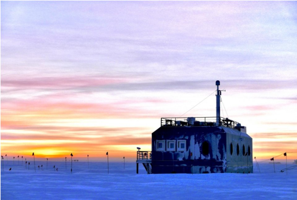
Left: NOAA's observatory at Barrow (Utqiaġvik), Alaska, on the Arctic coast. Photo: NOAA (public domain). Right: NOAA's Atmospheric Research Observatory at the South Pole. Photo: Ian Crocker, NOAA (public domain). Both via Wikimedia Commons.
If you restarted, run the setup cell, then the checkpoint cell below. It restores the two lists from Your turn 6 that every part uses.
# ── Checkpoint ── run this if you restarted the kernel or fell behind ──
season = ["sin_month", "cos_month"]     # the two seasonal columns, from Your turn 5
candidates = [["decades"] + season,     # the four candidates of Your turn 6
              ["decades", "decades2"] + season,
              ["decades", "decades2", "decades3"] + season,
              ["decades", "decades2", "decades3", "decades4"] + season]
names = ["line", "squared", "cubed", "fourth power"]
brw.head()
✏️ Your turn 10
Which curve do Barrow's validation years choose?
Why: class chose on Mauna Loa's validation decade. Barrow's record is shorter (it starts in 1973) and its teeth are bigger, so the choice could come out differently.
- The columns: add
decades2,decades3,decades4,sin_monthandcos_monthtobrw, as class did formlo. brw_trainingandbrw_validation: the months up to 2000, and 2001 to 2010.- The loop: for each list of columns in
candidates(the four column lists of Your turn 6, with their names innames), fit to Barrow's training months and append its validation RMSE tobrw_validation_rmses. brw_best: the name with the smallest validation RMSE.
Use these names, because the self-check looks for them: brw_validation_rmses and brw_best.
# ← your answer here: replace every ... with code
brw["decades2"] = ...   # the decades column, squared
brw["decades3"] = ...   # cubed
brw["decades4"] = ...   # to the fourth power
angle = 2 * np.pi * (brw["month"] - 0.5) / 12
brw["sin_month"] = ...  # the sine of each month's angle
brw["cos_month"] = ...  # the cosine

brw_training = ...    # Barrow's months up to the end of 2000
brw_validation = ...  # Barrow's months from 2001 to 2010

brw_validation_rmses = []
for columns in candidates:            # the four column lists of Your turn 6 (the checkpoint restores them)
    model = ...                       # this candidate, fitted to Barrow's training months
    residuals = ...                   # Barrow's validation months: data minus model
    brw_validation_rmses.append(...)  # the typical validation miss

brw_best = ...  # the name of the candidate with the smallest validation RMSE
for i in range(4):
    print(names[i], ": validation", round(brw_validation_rmses[i], 2), "ppm")
print("Barrow's validation months choose:", brw_best)
# Self-check: run this after your answer. You do not need to read it — it only says whether something is off.
assert [round(x, 2) for x in brw_validation_rmses] == [4.69, 3.23, 4.94, 19.3], "fit each candidate on Barrow's months up to 2000, score it on 2001-2010"
assert brw_best == "squared", "brw_best is the name with the smallest validation RMSE"
print(f"✓ Your turn 10 — Barrow's validation months choose the {brw_best} curve")
What the numbers mean. Does Barrow choose the same curve as Mauna Loa? Its record starts in 1973, so its training months are fewer. Which would you trust more if the two stations disagreed, and why?
✏️ Your turn 11
How well does Barrow's curve do on its test years, and how big is its yearly swing?
Why: Your turn 7 tested Mauna Loa's choice once; Your turn 9 measured Mauna Loa's swing. Do both for Barrow. Its swing is the question: is the Arctic's breath bigger or smaller than Hawaii's?
brw_test_rmse: refit Barrow's chosen columns (the entry ofcandidatesnamedbrw_best, the curve Barrow chose in Your turn 10) to its months up to 2010, then measure the miss on its months from 2011 on, and draw the test months with the curve.brw_swing,brw_peak,brw_low: fit the chosen columns to every Barrow month, then work out the seasonal part as in Your turn 9: its size, and the months of its high and its low.
Use these names, because the self-check looks for them: brw_test_rmse, brw_swing,
brw_peak and brw_low.
# ← your answer here: replace every ... with code
columns = candidates[names.index(brw_best)]  # the columns of the curve Barrow chose in Your turn 10
brw_before_test = ...                        # Barrow's months up to the end of 2010
brw_test = ...                               # Barrow's months from 2011 on
model = ...                                  # the chosen columns, fitted to the months before the test
residuals = ...                              # the test months: data minus model
brw_test_rmse = ...                          # the typical test miss

plt.figure(figsize=(8, 4))
plt.plot(brw[brw_test]["time"], brw[brw_test]["co2"], color="0.6", marker=".", label="data")
plt.plot(..., ..., label="chosen curve, fitted to Barrow up to 2010")  # the test months' time, and the curve's CO2 for them
plt.xlabel("year")
plt.ylabel("CO2 (ppm)")
plt.title("Barrow's test months")
plt.legend()
plt.show()

model = ...          # the chosen columns, fitted to every Barrow month
sine_weight = ...    # the number the fit found for the sine column
cosine_weight = ...  # the number the fit found for the cosine column
month_numbers = np.arange(1, 13)
month_angle = 2 * np.pi * (month_numbers - 0.5) / 12
seasonal_part = ...  # the yearly wave: the two weights times their waves, added
brw_swing = ...      # the wave's highest value minus its lowest
brw_peak = ...       # the month number of the highest value
brw_low = ...        # the month number of the lowest value
print("Barrow: test miss", round(brw_test_rmse, 2), "ppm; a yearly swing of", round(brw_swing, 1),
      "ppm, highest in month", brw_peak, "and lowest in month", brw_low)
# Self-check: run this after your answer. You do not need to read it — it only says whether something is off.
assert abs(brw_test_rmse - 3.84) < 0.01, "refit on Barrow's months up to 2010, measure on 2011 on"
assert round(brw_swing, 1) == 14.3 and (brw_peak, brw_low) == (3, 9), "fit every Barrow month, then the seasonal part as in Your turn 9"
print(f"✓ Your turn 11 — Barrow swings {brw_swing:.1f} ppm a year, highest in month {brw_peak}")
What the numbers mean. Compare Barrow's swing with Mauna Loa's (5.6 ppm). Barrow is in the far north, nearer the great northern forests and tundra. Why might its swing be bigger?
✏️ Your turn 12
Which curve does the South Pole choose, and how big is its swing?
Why: the South Pole is as far from the northern plants as a station can be. Repeat Your turns
10 and 11 there, in one cell: the columns, the choice among candidates (the four column lists
of Your turn 6), and the swing (no test this time). Each line is yours to write in full; the
comment beside it says what the line does, in the order of Your turns 10 and 11.
Use these names, because the self-check looks for them: spo_validation_rmses, spo_best,
spo_swing, spo_peak and spo_low.
# ← your answer here: replace every ... with code
spo["decades2"] = ...   # the decades column, squared
spo["decades3"] = ...   # cubed
spo["decades4"] = ...   # to the fourth power
angle = ...             # each month's angle, as for Barrow
spo["sin_month"] = ...  # the sine of each month's angle
spo["cos_month"] = ...  # the cosine

spo_training = ...                    # the South Pole's months up to the end of 2000
spo_validation = ...                  # the South Pole's months from 2001 to 2010
spo_validation_rmses = []
for columns in candidates:            # the four column lists of Your turn 6
    model = ...                       # this candidate, fitted to the training months
    residuals = ...                   # the validation months: data minus model
    spo_validation_rmses.append(...)  # the typical validation miss
spo_best = ...                        # the name of the candidate with the smallest validation RMSE
for i in range(4):
    print(names[i], ": validation", round(spo_validation_rmses[i], 2), "ppm")

columns = ...        # the columns of the curve the South Pole chose
model = ...          # those columns, fitted to every South Pole month
sine_weight = ...    # the number the fit found for the sine column
cosine_weight = ...  # the number the fit found for the cosine column
month_numbers = np.arange(1, 13)
month_angle = 2 * np.pi * (month_numbers - 0.5) / 12
seasonal_part = ...  # the yearly wave: the two weights times their waves, added
spo_swing = ...      # the wave's highest value minus its lowest
spo_peak = ...       # the month number of the highest value
spo_low = ...        # the month number of the lowest value
print("the South Pole chooses", spo_best, "; a yearly swing of", round(spo_swing, 1),
      "ppm, highest in month", spo_peak, "and lowest in month", spo_low)
# Self-check: run this after your answer. You do not need to read it — it only says whether something is off.
assert [round(x, 2) for x in spo_validation_rmses] == [3.15, 3.49, 1.65, 11.08], "the same loop as Your turn 10, on the South Pole's months"
assert spo_best == "cubed", "spo_best is the name with the smallest validation RMSE"
assert round(spo_swing, 1) == 1.0 and (spo_peak, spo_low) == (9, 3), "the seasonal part, from the chosen columns fitted to every month"
print(f"✓ Your turn 12 — the South Pole chooses the {spo_best} curve and swings {spo_swing:.1f} ppm")
What the numbers mean. The South Pole's swing peaks in a different half of the year from Barrow's. What is different about the seasons, and the land, in the southern half of the planet?
✏️ Your turn 13
How does the planet's breath change from north to south?
Why: three stations, three swings. Put them side by side, in order of latitude.
swings: a list of the three swings, Barrow, Mauna Loa, the South Pole, in that order (written at the top of the cell, as Your turns 9, 11 and 12 find them, so a slip there does not cost this part).- The figure: a bar for each station.
biggest: the name of the station with the biggest swing, found withnp.argmax.
Use these names, because the self-check looks for them: swings and biggest.
# ← your answer here: replace every ... with code
barrow_swing = 14.3     # ppm, what Your turn 11 finds
mauna_loa_swing = 5.6   # ppm, what Your turn 9 finds
south_pole_swing = 1.0  # ppm, what Your turn 12 finds
stations = ["Barrow (71° N)", "Mauna Loa (19.5° N)", "South Pole (90° S)"]
swings = ...            # the three swings, in the order of stations
biggest = ...           # the station at the position of the biggest swing

plt.figure(figsize=(7, 4))
plt.bar(..., ...)  # one bar per station: the names, then the swings
plt.xlabel("station")
plt.ylabel("yearly swing of CO2 (ppm)")
plt.title("The yearly breath, from north to south")
plt.show()
print("the biggest yearly swing is at", biggest)
# Self-check: run this after your answer. You do not need to read it — it only says whether something is off.
assert swings == [14.3, 5.6, 1.0], "the swings of Barrow, Mauna Loa and the South Pole, in that order"
assert biggest == "Barrow (71° N)", "biggest is the station at the position of the largest swing"
print(f"✓ Your turn 13 — the biggest yearly swing is at {biggest}")
What the numbers mean. The long rise is about the same at all three stations. The yearly swing is not. What does that tell you about where the swing comes from, and how fast the air mixes?
The whole planet at once. NOAA samples the air at dozens of sites from pole to pole. Its picture of every latitude together shows what your three stations found: a big yearly swing in the north, a small one in the tropics, almost none in the far south, and one long rise everywhere.
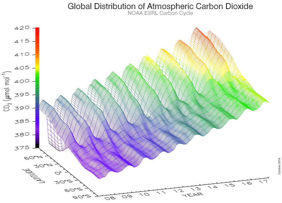
CO2 by latitude and year, 2008–2017, from NOAA's global sampling network. Figure: Ed Dlugokencky and Pieter Tans, NOAA (public domain), via Wikimedia Commons.