How long was the Earth frozen?
EPS 88 · PyEarth. Open your own copy on DataHub: click here.
In the mountains of northwest Canada, a layer of rock left by glaciers sits on older rock and under younger rock. Geologists think it records a time when ice spread over most of the planet, a "Snowball Earth". How long did the ice last? A rock layer does not come with a date written on it, but some of its atoms are a clock.
Today you read that clock with the line fit of the last two weeks: the slope of a line through a rock's measurements is its age. Then comes the question every age must answer before anyone should believe it: how sure is it? You answer that by letting the computer redraw your own measurements thousands of times. At home you read a new clock with the same steps.
Every place you write something opens with a pencil icon and the words Your turn, and is
followed by a cell that already has the shape of the answer written in, with ... wherever your
code goes. Replace every ..., run every cell so your answers and figures are
saved in the file, then download this notebook itself — the .ipynb file — and upload it
to Gradescope. Not a PDF: the marking reads your notebook, and a PDF cannot be read.
In JupyterLab: File ▸ Download, or right-click the file in the left-hand panel and choose
Download.
Two habits from the first minute. A cell runs when you press Shift+Enter, and the notebook remembers everything it has already run — so when something breaks and you cannot see why, Kernel → Restart Kernel and Run All Cells throws the memory away and rebuilds it from the top. That is never the wrong thing to do.
What you'll be able to do
The science. Explain how a rock records its own age; read an age from an isochron; say how long the Sturtian Snowball Earth lasted and how sure that number is; and say why a published age carries a "±".
The code. A line fit with LinearRegression, and an age from its slope with np.log · a new
table drawn from an old one with table.sample(..., replace=True) · the bootstrap: redraw, refit,
repeat · a 95% interval with np.percentile.
Thirteen places where you write something: nine in class, four at home, the last two
optional. Each is headed
Your turn, and the cell under it has the shape of the answer written in, with ... wherever
your code goes and a comment beside each one saying what goes there.
The three questions of the class:
- How can a rock tell its own age?
- How sure is an age from 37 samples?
- How long was the Earth frozen?
Setup
Run the next cell once. It reads four tables stored with the course, each one a published measurement, one row per sample:
rocks: 37 samples of the granite-like rocks of the Monterey Peninsula, California (Kistler and Champion, US Geological Survey, 2001). The columnmaterialsays whether a sample is a piece of the whole rock (33) or crystals of feldspar separated from it (4);cap: the rock just above the Snowball Earth glacial deposits in northwest Canada (Rooney and others, 2014). The columncollected_fromsays where each sample came from: one thin bed, or 6 m of rock;far_sideandfossil_layer: the two tables for the homework.
Every table has the same two measurement columns, parent and daughter. Each is a ratio of
two kinds of atom, not a count; part 1 explains which atoms.
Ages are in millions of years ago, written Ma.
import numpy as np
from sklearn.linear_model import LinearRegression
import pandas as pd
import matplotlib.pyplot as plt

# house style, set once, so every plot cell below holds only what matters
plt.rcParams.update({"figure.dpi": 110,
                     "axes.grid": True, "grid.alpha": 0.3, "axes.axisbelow": True})

CACHE = "https://raw.githubusercontent.com/AI4EPS/EPS88_PyEarth/main/data"

rocks = pd.read_csv(CACHE + "/week08_monterey_rbsr.csv")       # Monterey granite: one row per sample
cap = pd.read_csv(CACHE + "/week08_snowball_reos.csv")         # Snowball Earth: the rock above the glacial deposits
far_side = pd.read_csv(CACHE + "/week08_change6_rbsr.csv")     # homework: lava from the far side of the Moon
fossil_layer = pd.read_csv(CACHE + "/week08_nadaleen_j1719_reos.csv")  # homework: a layer from the age of the first large organisms
rb_decay = 1.42e-11     # the share of rubidium-87 atoms that decay each year
re_decay = 1.666e-11    # the share of rhenium-187 atoms that decay each year
print(len(rocks), "Monterey samples and", len(cap), "Snowball Earth samples")
1. How can a rock tell its own age?
The question. About 717 million years ago, glaciers spread over what is now northwest Canada, which then lay at the equator: ice reached the sea in the tropics (Macdonald and others, 2010). The Snowball Earth hypothesis (Kirschvink, 1992) says ice covered nearly the whole planet:
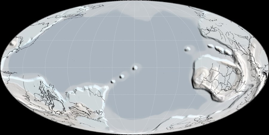
One reconstruction of the Earth 690 million years ago, with ice (white) over the land and the sea. Map: C. R. Scotese and others, PALEOMAP Project, Wikimedia Commons (CC BY 4.0).
In the Mackenzie Mountains of northwest Canada the glacial deposits of this ice age, the Sturtian, are the Rapitan Group, and right on top of them lies a cap of dark limestone, the base of the Twitya Formation, laid down in the sea as the ice ended:
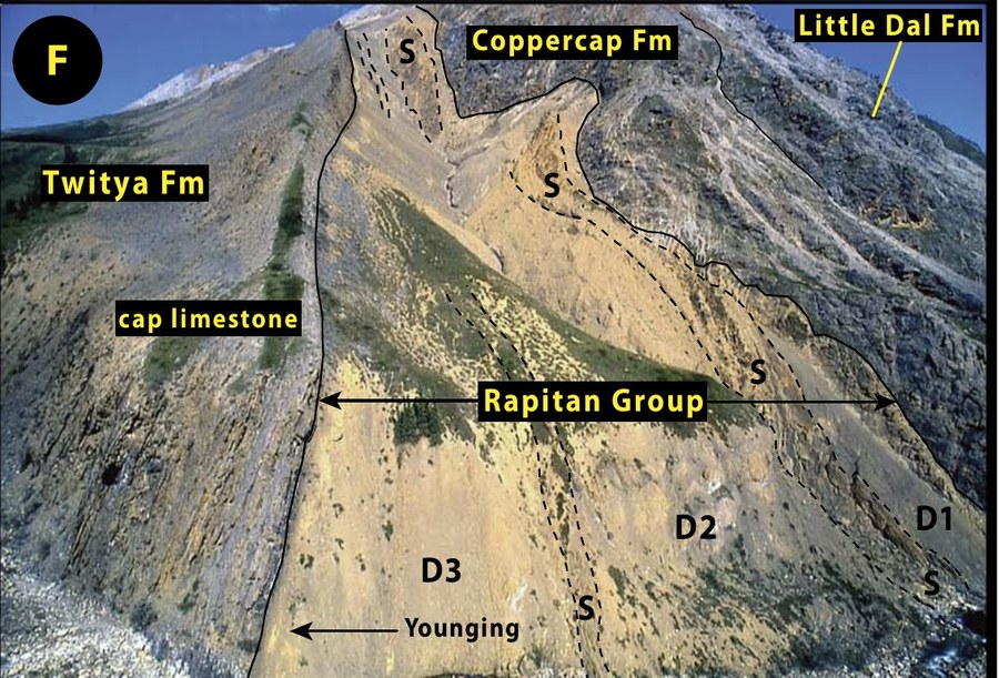
The Rapitan Group (D1 to D3: rock laid down under ice; S: layered) and the cap limestone of the Twitya Formation, Mackenzie Mountains, Northwest Territories, Canada. Figure: Hoffman and others (2017), Science Advances, Fig. 19F (CC BY-NC 4.0).
How do we know ice made these rocks? Stones carried by floating ice dropped into soft mud on the sea floor and bent its layers, something only ice does in a quiet sea:
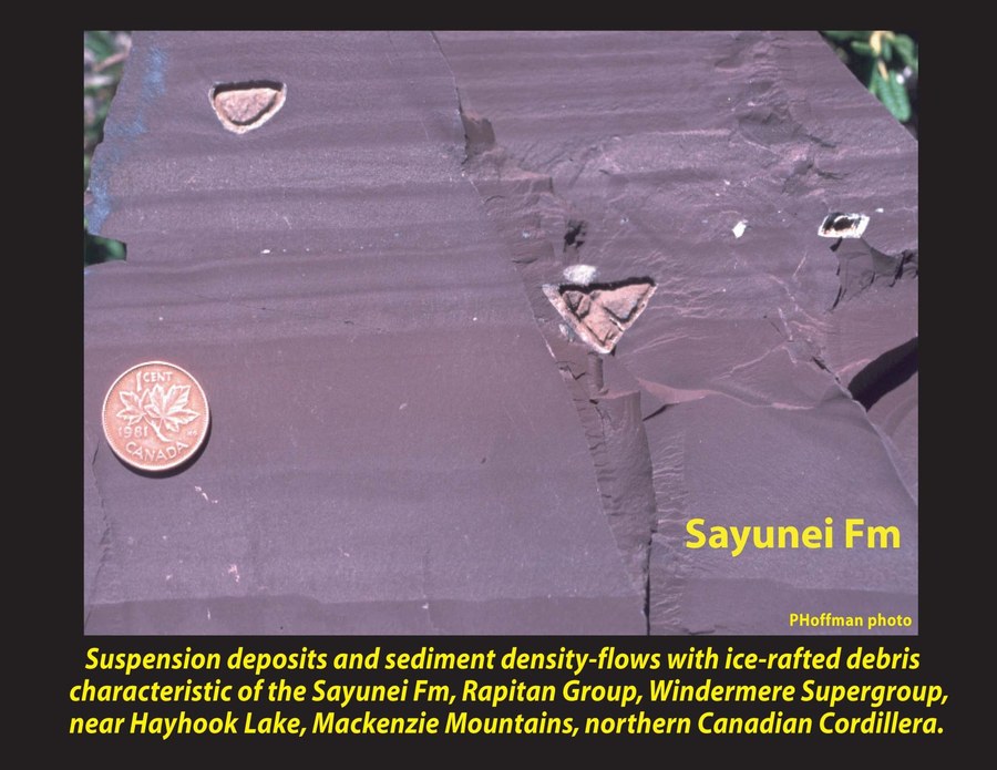
Stones dropped from floating ice into mud, Sayunei Formation of the Rapitan Group, with a coin for scale. Photo: P. F. Hoffman, snowballearth.org.
When did the ice begin, and when did it end? The start is known: a layer of volcanic ash inside the glacial deposits of the Yukon, dated with the uranium-lead clock, is 716.5 million years old, so the ice was there by then. That ash was dated by Francis Macdonald, now a professor in this department, and his colleagues (Macdonald and others, 2010). The end is the age of the cap limestone, and that is what you will measure. The plan: learn how a rock's clock works, read it on a rock with many samples (the granite of Monterey, part 2), then read it on the cap, which has only 7 (part 3).
What the numbers in "strontium-87" mean. An atom has a small nucleus made of protons and neutrons. The number of protons decides which element it is: every rubidium atom has 37, every strontium atom 38. The number after the name is the mass number, protons plus neutrons:
| Atom | Protons | Neutrons | Mass number |
|---|---|---|---|
| strontium-86 | 38 | 48 | 86 |
| strontium-87 | 38 | 49 | 87 |
| rubidium-87 | 37 | 50 | 87 |
Strontium-86 and strontium-87 are isotopes: the same element, with different numbers of neutrons. Isotopes of one element behave the same way in chemistry, so a crystal growing in a magma takes up strontium-86 and strontium-87 in the same proportion as the magma around it. That is why every mineral of one rock starts with the same 87Sr/86Sr.
Rubidium-87 is radioactive: in its nucleus one neutron turns into a proton and an electron flies out. The atom now has 38 protons, so it is strontium, and still 87 protons plus neutrons: rubidium-87 has become strontium-87. That is why the parent and the daughter share the number 87.
Some atoms are clocks. A parent atom, such as rubidium-87, turns by itself into a daughter atom, strontium-87. Nothing speeds it up or slows it down: no heat, no pressure. Each year the same small share of the parent atoms that are left decays, so the number left falls along a curve like this one. The half-life is the time it takes for half of the parent atoms to decay, however many there are.
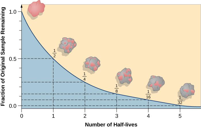
The share of the parent left after each half-life. Figure: Fraknoi, Morrison and Wolff, Astronomy (OpenStax), CC BY 4.0.
How the clock runs: by halving. After one half-life, half the parent atoms are left; after two, half of that half, a quarter; after three, an eighth. After any time $t$:
$$\frac{N}{N_0} = \left(\frac{1}{2}\right)^{t / T_{1/2}}$$
where $N_0$ is the number of parent atoms at the start, $N$ the number left now, and $T_{1/2}$ the half-life.
The same law, written with the decay rate. The same curve is usually written with the share
of the parent that decays each year, the decay rate $\lambda$ (lambda): for rubidium-87, 1.42
in every hundred billion atoms a year, rb_decay in the setup cell.
$$N = N_0 \, e^{-\lambda t}, \qquad \lambda = \frac{\ln 2}{T_{1/2}}$$
Here $e = 2.718\ldots$; np.exp(x) computes $e^x$ (the probability week), and np.log(x), the
natural logarithm $\ln x$, undoes it: np.log(np.exp(x)) is x.
✏️ Your turn 1
Do the two laws agree, and how fast does the rubidium clock run?
Why: the two forms of the decay law must give the same share left; then the age of the Earth shows how slow this clock is.
halving: the share left after time $t$ by the halving law, $(1/2)^{t / T_{1/2}}$.left: the share left by the decay-rate law, $e^{-\lambda t}$, withnp.exp.decayed: the share decayed after time $t$, $1 - e^{-\lambda t}$.
In the loops t is the time $t$, in years.
Use these names, because the self-check looks for them: left and decayed.
# ← your answer here: replace every ... with code
half_life = np.log(2) / rb_decay  # T½ = ln 2 / λ, in years
print("half-life of rubidium-87:", round(half_life / 1e9, 1), "billion years")
for t in [1 * half_life, 2 * half_life, 3 * half_life]:
    halving = ...                 # N / N0 = (1/2)^(t / T½)
    left = ...                    # N / N0 = e^(−λt): the share left
    print(round(t / half_life), "half-lives: (1/2)^(t/T½) =", round(halving, 4), " e^(−λt) =", round(left, 4))
for t in [83.5e6, 4.5e9]:
    decayed = ...                 # the share decayed: 1 − e^(−λt)
    print("after", t / 1e6, "million years,", round(100 * decayed, 2), "% of the rubidium-87 has decayed")
# Self-check: run this after your answer. You do not need to read it — it only says whether something is off.
assert round(left, 4) == 0.125, "left = np.exp(-rb_decay * t): after three half-lives an eighth is left"
assert round(100 * decayed, 2) == 6.19, "decayed = 1 - np.exp(-rb_decay * t), for t = 4.5e9 years"
print(f"✓ Your turn 1 — the two laws agree; in 4.5 billion years {100 * decayed:.2f}% of the rubidium-87 has decayed")
A slow clock. In the 83.5 million years since the Monterey rocks formed, only 0.12% of their rubidium-87 has decayed; even in the 4.5 billion years of the Earth's life, only 6.19%. So the daughter ratios of the Monterey rocks differ only in the third decimal place, and reading an age takes very careful measurements, made in laboratories like this one:
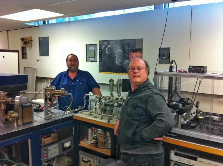
The argon lab of the Berkeley Geochronology Center, where rock ages like these are measured. Photo: Berkeley Geochronology Center.
Ages answer other questions too. Clocks like this showed that the dinosaurs died out at the same time as an asteroid struck Mexico 66 million years ago, the two ages agreeing to within 32,000 years; the team was led by Paul Renne, a professor in this department and director of the Berkeley Geochronology Center (Renne and others, 2013). The search for that impact began at a thin layer of clay in Italy:
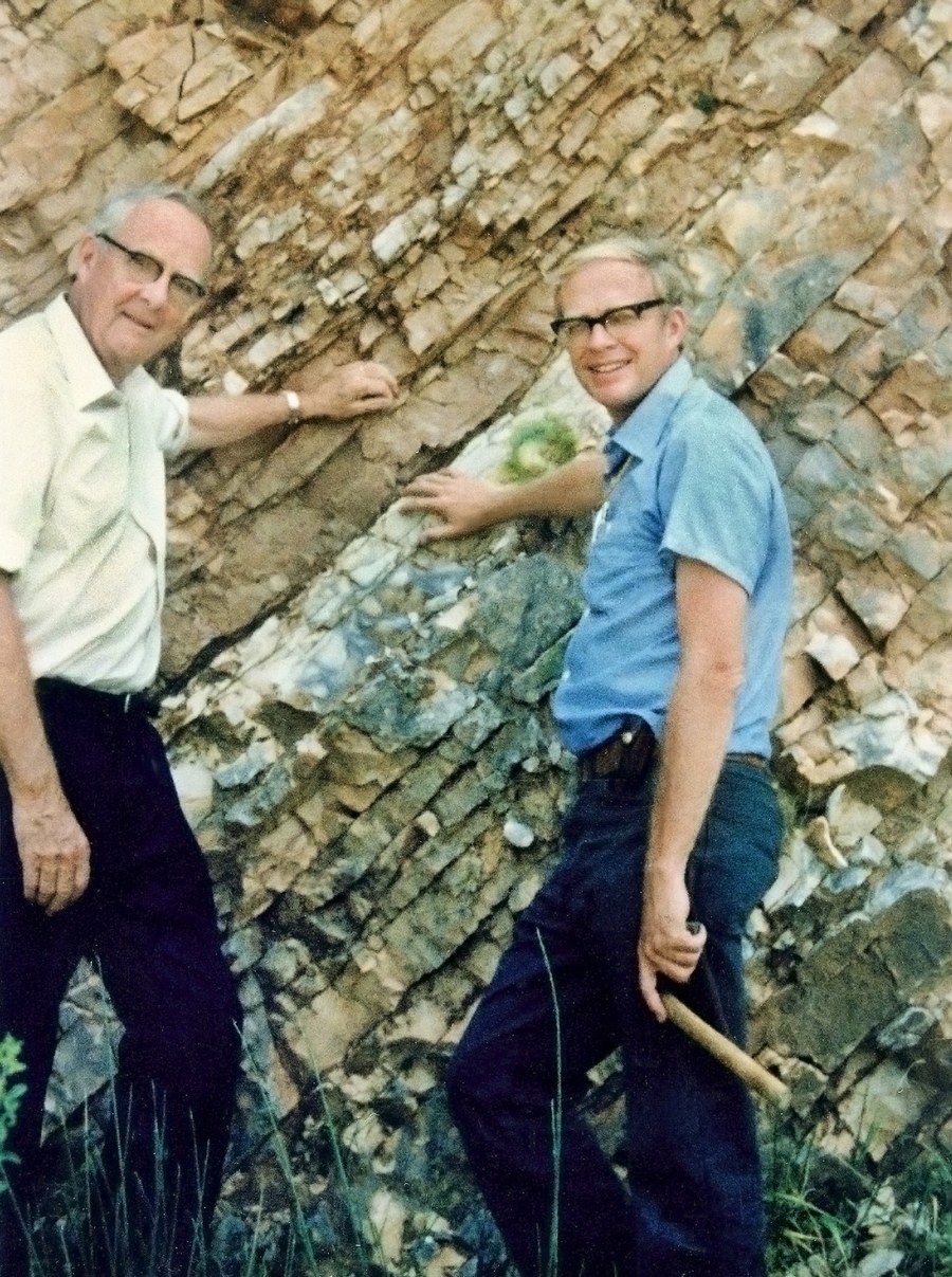
Luis Alvarez and his son Walter Alvarez, both of Berkeley, at the thin layer that marks the dinosaurs' extinction, near Gubbio, Italy; Walter Alvarez is still a professor in this department. Photo: Lawrence Berkeley Laboratory (public domain).
Back to Snowball Earth: how do the clock's atoms become two columns of numbers?
Three atoms, two ratios. The rubidium clock involves three kinds of atom in every mineral:
| Atom | Its role | Over time |
|---|---|---|
| rubidium-87 (87Rb) | the parent: radioactive | slowly decreases, as it turns into strontium-87 |
| strontium-87 (87Sr) | the daughter | some was there when the mineral formed; more is added as 87Rb decays |
| strontium-86 (86Sr) | the reference: a stable strontium atom | never changes: no decay makes or destroys it |
A laboratory cannot easily count atoms, but it can measure the ratio of two atoms very precisely. So everything is measured against strontium-86, the atom that never changes. Dividing by it also compares every mineral for the same amount of strontium, whatever its size. That gives the two columns of the table:
parent= 87Rb/86Sr: how much parent a mineral has, per atom of the reference;daughter= 87Sr/86Sr: how much daughter it has now, per atom of the reference.
A mineral rich in rubidium has a large parent and, as time passes, makes the most new
strontium-87, so its daughter climbs fastest.
From parent to daughter. Every parent atom that decays becomes one daughter atom, so the daughter made is the parent lost. We can measure the parent left today, $N$, but not the parent at the start; turning the decay law round, $N_0 = N e^{\lambda t}$, so
$$D^{*} = N_0 - N = N \left(e^{\lambda t} - 1\right)$$
and a mineral's daughter today, $D$, is what it started with, $D_0$, plus what was made:
$$D = D_0 + N \left(e^{\lambda t} - 1\right)$$
One rock, many minerals, one line. The minerals of a rock take in different amounts of the parent when they grow, but the same ratio of daughter. So at the start they sit on a flat line; as the parent decays, each gains daughter in proportion to its parent, and the line tilts more every year. That line is an isochron ("same time"): minerals that formed together started with the same daughter atoms; each has since gained more in proportion to its parent atoms, so together they lie on a line whose slope grows with time.
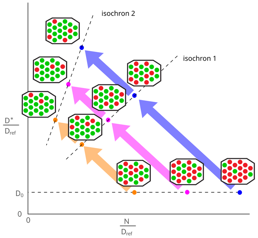
Three minerals of one rock (orange, pink, blue) start on the flat line D0. As parent atoms (red) turn into daughter atoms (green), each moves up and to the left, and the line through them steepens: isochron 1, then isochron 2. Figure: Woudloper, Wikimedia Commons (CC BY-SA 4.0).
The isochron equation. Divide every term of $D = D_0 + N(e^{\lambda t} - 1)$ by the strontium-86
of the mineral: $D$ becomes the daughter ratio, $D_0$ the ratio the mineral started with, and $N$
the parent ratio:
$$\frac{^{87}\mathrm{Sr}}{^{86}\mathrm{Sr}} = \left(\frac{^{87}\mathrm{Sr}}{^{86}\mathrm{Sr}}\right)_0 + \left(e^{\lambda t} - 1\right) \frac{^{87}\mathrm{Rb}}{^{86}\mathrm{Sr}}$$
In words: daughter now = daughter at the start + parent × (e^(λt) − 1). This is a straight
line, $y = \text{intercept} + \text{slope} \times x$, with $x$ = parent and $y$ = daughter.
Every mineral of one rock started with the same daughter ratio (the intercept) and has aged the
same time $t$ (so the same slope, $e^{\lambda t} - 1$), so they all lie on one line.
First, a rock with many samples: the Monterey Peninsula. The rocky coast from Monterey to Point Lobos is a granite-like rock that cooled from magma deep underground. Close up it is a mix of crystals of different minerals, and each mineral took in a different amount of rubidium when it grew:
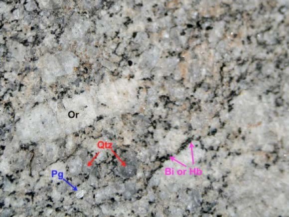
The Monterey granodiorite close up: pink-white feldspar crystals (Or, Pg), grey quartz (Qtz) and dark mica and hornblende (Bi, Hb). Photo: E. Clifton, Rocks of Point Lobos (2013).
These rocks sit on a long block of crust just west of the San Andreas fault, the Salinian block. It is out of place: many geologists think it formed far to the south-east, beside the southern Sierra Nevada, and was carried north-west along the fault, about 300 km on the San Andreas alone (Ross, 1984); where exactly it came from is still debated. Its age is one of the clues.
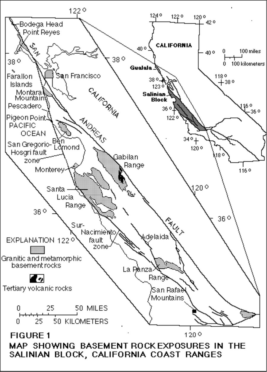
The granite-like rocks of the Salinian block (dark), between the San Andreas fault and the coast. Map: Kistler and Champion (2001), US Geological Survey (public domain).
Monterey gives 37 samples, enough to learn the method on; the Snowball cap gives 7. The Monterey table:
rocks.head()
Check the equation on two real samples. The report says these rocks formed 83.5 million years ago with a daughter ratio of 0.70787. Take the samples with the least parent (0.26, sample SANLU9-90) and the most (3.59, SANLU1B-94), and predict their daughter ratio today:
t = 83.5e6                          # years: the report's age
D0 = 0.70787                        # D0: the daughter ratio when the rocks formed (the report's value)
growth = np.exp(rb_decay * t) - 1   # e^(λt) − 1: new strontium-87 made per rubidium-87 atom
D_low = D0 + 0.26 * growth          # D = D0 + N (e^(λt) − 1), with N = 0.26: sample SANLU9-90, the least parent
D_high = D0 + 3.59 * growth         # the same, with N = 3.59: sample SANLU1B-94, the most parent
print("e^(λt) − 1 =", round(growth, 6))
print("least parent: predicted", round(D_low, 5), "measured 0.70841")
print("most parent:  predicted", round(D_high, 5), "measured 0.71203")
The sample with 14 times more parent has gained 14 times more strontium-87, and both predictions land within about 0.0002 of what was measured. That small difference is the scatter of real samples about the line.
✏️ Your turn 2
Do the Monterey rocks lie on a line?
Why: an age needs a line. Look before you fit.
- The figure: one dot per rock, the
parentcolumn across and thedaughtercolumn up.
Use the names in the cell, so later cells can read them.
# ← your answer here: replace every ... with code
plt.figure(figsize=(7, 5))
...  # a scatter plot of rocks: the parent column across, the daughter column up
plt.xlabel("parent: rubidium-87 / strontium-86")
plt.ylabel("daughter: strontium-87 / strontium-86")
plt.title(f"Monterey: {len(rocks)} samples")
plt.show()
The rocks lie close to a rising line, with some scatter about it. The rocks with more parent have more daughter: the clock has been running. The steeper the line, the older the rock.
2. How sure is an age from 37 samples?
On Monterey's 37 samples you learn the two skills the 7-sample Snowball cap will need in part 3: reading the clock, and saying how sure the reading is.
From the line to the age, step by step. Part 1 ended with the isochron equation:
$$\text{daughter now} = \text{daughter at the start} + \left(e^{\lambda t} - 1\right) \times \text{parent}$$
The line you will fit in Your turn 3 has the same shape:
$$\text{daughter} = \hat{a} + \hat{b} \times \text{parent}$$
A hat marks a number fitted from the data. Match them term by term: the intercept $\hat{a}$ is the daughter ratio at the start, and the slope $\hat{b}$ is $e^{\lambda t} - 1$. Add 1, take the natural log (ln undoes e), divide by $\lambda$:
$$\hat{b} = e^{\lambda t} - 1 \quad\Rightarrow\quad e^{\lambda t} = 1 + \hat{b} \quad\Rightarrow\quad t = \frac{\ln(1 + \hat{b})}{\lambda}$$
With the Monterey numbers you are about to get: $\hat{b}$ is 0.0011749, so $1 + \hat{b}$ is
1.0011749; its natural log is 0.0011742; divided by 1.42e-11 per
year, that is 82.7 million years. In code, the three
steps are one line, with b for $\hat{b}$: np.log(1 + b) / rb_decay.
✏️ Your turn 3
How old is the Monterey granite?
Why: the line fit of the last two weeks, with a new meaning for its slope.
model: a straight line fitted to the rocks, theparentcolumn (as a table, double brackets) to thedaughtercolumn, as in the line-fitting week.b: its slope, $\hat{b}$:model.coef_[0], as in the line-fitting week.age_ma: the age, $t = \ln(1 + \hat{b}) / \lambda$, in millions of years:np.log(1 + b)overrb_decay, then over a million.- The figure: the rocks as dots and the fitted line through them, drawn with
model.predict.
Use these names, because the self-check looks for them: b and age_ma.
# ← your answer here: replace every ... with code
model = LinearRegression().fit(..., ...)  # the parent column as a table, then the daughter column
b = ...                                   # b̂: the slope of the fitted line
age_ma = ... / rb_decay / 1e6             # t = ln(1 + b̂) / λ: the ... is ln(1 + b̂); / 1e6 for millions of years
print("slope", round(b, 7), "so the age is", round(age_ma, 1), "million years")

plt.figure(figsize=(7, 5))
plt.scatter(rocks["parent"], rocks["daughter"])
...  # the fitted line in red: the parent column across, ŷ = â + b̂ × parent up: the line's daughter at each rock's parent
plt.xlabel("parent: rubidium-87 / strontium-86")
plt.ylabel("daughter: strontium-87 / strontium-86")
plt.title(f"Monterey isochron: {age_ma:.1f} million years")
plt.show()
# Self-check: run this after your answer. You do not need to read it — it only says whether something is off.
assert round(age_ma, 1) == 82.7, "fit parent (double brackets) to daughter; b = model.coef_[0]; the age is np.log(1 + b) / rb_decay / 1e6"
print(f"✓ Your turn 3 — the Monterey granite is {age_ma:.1f} million years old")
82.7 million years. The geologists who measured these rocks reported 83.5 ± 6.2 million years, from the same table with a fit that also weighs each measurement's error.
Why the "± 6.2" matters as much as the 83.5. The same report dates these rocks with a second, different clock (argon in one of their minerals, hornblende) and gets 80.2 ± 0.5 million years. Is that a different age, or the same age measured twice? The numbers 83.5 and 80.2 alone cannot say. With their uncertainties they can: 83.5 ± 6.2 runs from 77.3 to 89.7, and 80.2 lies inside it, so the two clocks agree; the authors say they "overlap within experimental error" (Kistler and Champion, 2001). Every comparison of two numbers from data, two ages, two rates, a forecast and what happened, needs the uncertainty of each.
The "±" decides arguments, about Snowball Earth too. Did the ice melt at the same moment all over the world? The cap above the glacial deposits has been dated in three places:
| Place | Age of the cap (million years) |
|---|---|
| northwest Canada (Rooney and others, 2014) | 662.4 ± 3.9 |
| South Australia (Cox and others, 2018) | 663.03 ± 0.76 |
| Mongolia (Rooney and others, 2015) | 659.0 ± 4.5 |
Without the "±", 662.4, 663.0 and 659.0 look like three different thaws, millions of years apart. With it, every pair overlaps, so one thaw at the same time everywhere fits the data, which is now the common view (Hoffman and others, 2017).
Where does a "±" come from? We cannot go back to Monterey and collect 37 new rocks a thousand times. But we can ask the rocks we have.
The bootstrap. Ask the data the same question a thousand times, using a different random slice of itself each time. Draw 37 samples from our 37, at random and with
replacement: after each draw the rock goes back, so it can be drawn again. Some rocks come out
twice, some not at all. Fit the line again: a slightly different line, a slightly different age.
table.sample(n, replace=True, random_state=rng) makes one such draw from a table.
First, a case with a known answer. The mean of the 37 parent values has a textbook
uncertainty, its standard error $\sigma / \sqrt{n}$, with $\sigma$ the standard deviation of the
values. Redraw the 37 rocks 10,000 times and take the mean parent of each redraw: the spread of
those means should match the formula.
rng = np.random.default_rng(88)
redrawn_means = []
for i in range(10000):
    redrawn = rocks.sample(len(rocks), replace=True, random_state=rng)
    redrawn_means.append(np.mean(redrawn["parent"]))
print("spread of the 10,000 redrawn means:", round(np.std(redrawn_means), 3))
print("formula, σ / √n:                   ", round(np.std(rocks["parent"]) / np.sqrt(len(rocks)), 3))
The two agree: redrawing the samples we have reproduces the uncertainty the formula gives. The same redrawing works for any number computed from the samples, including an age, which comes from a slope and a logarithm.
✏️ Your turn 4
What does one redrawn set of rocks say?
Why: see one redraw before doing ten thousand.
resample: 37 rows drawn fromrockswith replacement, using the generatorrng.resample_age: the age from a line fitted toresample, by the steps of Your turn 3.
Use these names, because the self-check looks for them: resample and resample_age.
# ← your answer here: replace every ... with code
rng = np.random.default_rng(88)
resample = rocks.sample(..., replace=True, random_state=rng)  # as many rows as rocks has
print(len(resample["sample"].value_counts()), "different rocks among the", len(resample), "drawn")
resample_model = LinearRegression().fit(..., ...)             # the redrawn parent column as a table, then its daughter column
b = ...                                                       # b̂: this line's slope
resample_age = ... / rb_decay / 1e6                           # t = ln(1 + b̂) / λ, in millions of years
print("this redraw gives", round(resample_age, 1), "million years")
# Self-check: run this after your answer. You do not need to read it — it only says whether something is off.
assert len(resample) == 37 and round(resample_age, 1) == 80.9, "draw len(rocks) rows with replace=True and random_state=rng, then fit and convert as in Your turn 3"
print(f"✓ Your turn 4 — one redraw gives {resample_age:.1f} million years")
24 different rocks among 37: the rest are repeats. The redrawn samples give 80.9 million years instead of 82.7. One redraw is one other set of rocks the granite could have given us. Ten thousand show how far the age could wander.
✏️ Your turn 5
How far does the age wander over 10,000 redraws?
Why: the spread of the redrawn ages is the uncertainty of the age.
- The loop: start a generator from the seed 88; 10,000 times draw a
resampleas in Your turn 4, fit it, and append its age toboot_ages. age_range: the 2.5th and 97.5th percentiles ofboot_ages, withnp.percentile: the middle 95% of the ages lie between them.- The figure: a histogram of
boot_ages; the black lines at the ends ofage_rangeare drawn for you.
Use these names, because the self-check looks for them: boot_ages and age_range.
# ← your answer here: replace every ... with code
rng = np.random.default_rng(88)
boot_ages = []
for i in range(10000):
    resample = ...                           # 37 samples drawn from rocks with replacement, as in Your turn 4
    resample_model = ...                     # a line fitted to the redrawn samples
    b = ...                                  # b̂: this line's slope
    boot_ages.append(...)                    # t = ln(1 + b̂) / λ, in millions of years
age_range = np.percentile(..., [2.5, 97.5])  # the redrawn ages
print("95% confidence interval:", age_range.round(1), "million years")

plt.figure(figsize=(8, 4))
...                                       # a histogram of boot_ages, 50 bins
plt.axvline(age_range[0], color="black")  # the low end of the interval
plt.axvline(age_range[1], color="black")  # the high end
plt.xlabel("age of a redrawn set of rocks (millions of years)")
plt.ylabel("number of redraws")
plt.title("10,000 redraws of the Monterey samples; the black lines hold the middle 95%")
plt.show()
# Self-check: run this after your answer. You do not need to read it — it only says whether something is off.
assert [round(x, 1) for x in age_range] == [76.9, 89.8], "seed 88; each time sample len(rocks) rows with replace=True and random_state=rng; then the 2.5th and 97.5th percentiles"
print(f"✓ Your turn 5 — the age is between {age_range[0]:.1f} and {age_range[1]:.1f} million years (95%)")
82.7 million years, with a 95% interval of 76.9 to 89.8. That range is a confidence interval: not one number but the range your number would have wandered over, had the world rolled differently. It is about ± 6.4, close to the published ± 6.2, which the geologists worked out another way, from each rock's measurement error.
Back to the question of the two clocks. The argon age, 80.2, lies inside your interval too, so your own bootstrap says the same: the two clocks agree, and the gap between 82.7 and 80.2 is within the uncertainty of the age.
Seen as lines. Each redraw is a different line through the same cloud of rocks. A hundred of them, drawn together:
rng = np.random.default_rng(88)
plt.figure(figsize=(7, 5))
for i in range(100):
    redrawn = rocks.sample(len(rocks), replace=True, random_state=rng)
    redrawn_model = LinearRegression().fit(redrawn[["parent"]], redrawn["daughter"])
    plt.plot(rocks["parent"], redrawn_model.predict(rocks[["parent"]]), color="tab:blue", alpha=0.05)
plt.scatter(rocks["parent"], rocks["daughter"], color="black", zorder=3)
plt.xlabel("parent: rubidium-87 / strontium-86")
plt.ylabel("daughter: strontium-87 / strontium-86")
plt.title("100 redrawn lines: their spread is the uncertainty of the slope")
plt.show()
The lines cross near the middle of the cloud and fan out at its ends: the slope, and so the age, is held mostly by the rocks with the most and the least parent.
What does "95%" mean? It is a promise about the method: of many intervals made this way, about 19 in 20 should hold the true age. We can test the promise on real rocks. Pretend the geologists had collected only 10 of the 37. Bootstrap those 10, and see whether their interval holds the age from all 37. Then do it again with another 10, 25 times:
full_age = 82.7     # million years: the age from all 37 samples, Your turn 3
rng = np.random.default_rng(88)
plt.figure(figsize=(8, 6))
hits = 0
for row in range(25):
    small_set = rocks.sample(10, random_state=rng)     # 10 different rocks, as if no others were collected
    small_ages = []
    for i in range(1000):
        resample = small_set.sample(10, replace=True, random_state=rng)
        small_model = LinearRegression().fit(resample[["parent"]], resample["daughter"])
        b = small_model.coef_[0]
        small_ages.append(np.log(1 + b) / rb_decay / 1e6)
    low, high = np.percentile(small_ages, [2.5, 97.5])
    holds = (low <= full_age) & (full_age <= high)
    hits = hits + holds
    plt.plot([low, high], [row, row], color="tab:blue" if holds else "tab:red", linewidth=3)
plt.axvline(full_age, color="black", linestyle="--")
plt.xlabel("age (millions of years)")
plt.ylabel("one set of 10 samples")
plt.title(f"{hits} of 25 intervals hold the age from all 37 samples")
plt.show()
24 of 25 intervals hold the age from all 37 samples, near the promised 19 in 20. The red one missed: an unlucky set of 10. And the intervals are wide, 15 to 121 million years from end to end, because 10 samples say less than 37. An interval is honest about its own data: fewer rocks, wider interval.
The same question, answered by a formula. For a line fitted by least squares, the slope's
uncertainty also has an exact formula, with no redrawing. Think of each sample as a point on the
true line plus a small error, $y_i = a + b\,x_i + \varepsilon_i$ (with $x_i$ its parent, $y_i$ its
daughter); its residual $e_i = y_i - \hat{y}_i$, how far it sits above (+) or below (−) the fitted
line $\hat{y}_i = \hat{a} + \hat{b}\,x_i$, is what we can see of that error. A hat marks a number fitted
from the data. Three numbers, in three steps:
1. How noisy are the samples? The typical size of a residual, the spread:
$$s = \sqrt{\frac{\sum_i e_i^2}{n - 2}}$$
(divided by $n - 2$, not $n$, because the slope and the intercept were already fitted from the same $n$ samples).
2. How far apart are the samples along the $x$ axis? With $\bar{x}$ their mean:
$$S_{xx} = \sum_i (x_i - \bar{x})^2$$
3. How uncertain is the slope? Noise over spread, the slope's standard error:
$$\mathrm{SE}(\hat{b}) = \frac{s}{\sqrt{S_{xx}}}$$
Picture a ruler laid through points that each wobble up or down by about $s$. If the points sit close together, a small wobble tips the ruler a lot; if they are far apart, the same wobble hardly tips it. So more noise makes the slope less certain, and samples spread farther along the line make it more certain.
The 95% interval is then $\hat{b} \pm t_{95} \times \mathrm{SE}(\hat{b})$, with $t_{95}$ from a table for $n - 2$ degrees of freedom: 2.0301 for 37 samples. With many samples $t_{95}$ is close to 2 (the familiar "± 2 standard errors"); with few, it is larger, because $s$ itself is then only a rough estimate and the interval must allow for that. The age interval is the ages of the two ends. The formula assumes the errors are independent and of about the same size along the line.
✏️ Your turn 6
What does the formula say about the Monterey age?
Why: a second, independent way to the same interval, to check the bootstrap.
Each name is a symbol in the math: b is $\hat{b}$, e is $e_i$, s is $s$, Sxx is $S_{xx}$,
SE_b is $\mathrm{SE}(\hat{b})$, t95 is $t_{95}$, and b_ends holds $\hat{b} \pm t_{95}\,\mathrm{SE}(\hat{b})$.
bande: the slope ofmodel(Your turn 3), and each sample'sdaughterminus the line's prediction for it.s,SxxandSE_b: steps 1, 2 and 3 above.b_ends: the two ends, $\hat{b} \pm t_{95}\,\mathrm{SE}(\hat{b})$, in one array; the given last line turns them into ages.
Use these names, because the self-check looks for them: SE_b and formula_range.
# ← your answer here: replace every ... with code
b = ...                                              # b̂: the slope of model (Your turn 3)
e = ...                                              # e_i = y_i − ŷ_i: each daughter minus the fitted line's daughter at its parent
s = ...                                              # s = √( Σ e_i² / (n − 2) ), with n = len(e)
Sxx = ...                                            # S_xx = Σ (x_i − x̄)², with x the parent column of rocks
SE_b = ...                                           # SE(b̂) = s / √S_xx
t95 = 2.0301                                         # t_95 from the t-table: n − 2 = 35 degrees of freedom
b_ends = ...                                         # b̂ ± t_95 × SE(b̂): the lower and the upper end, as one array
formula_range = np.log(1 + b_ends) / rb_decay / 1e6  # t = ln(1 + b̂) / λ at each end, in millions of years
print("slope", round(b, 7), "± standard error", round(SE_b, 7))
print("formula: 95% interval", formula_range.round(1), "million years")
# Self-check: run this after your answer. You do not need to read it — it only says whether something is off.
assert f"{SE_b:.3g}" == "4.78e-05", "SE_b = s / np.sqrt(Sxx), with s = np.sqrt((e ** 2).sum() / (len(e) - 2))"
assert [round(x, 1) for x in formula_range] == [75.9, 89.5], "b_ends = np.array([b - t95 * SE_b, b + t95 * SE_b])"
print(f"✓ Your turn 6 — the formula gives {formula_range[0]:.1f} to {formula_range[1]:.1f} million years")
The formula: 75.9 to 89.5 million years. The bootstrap: 76.9 to 89.8. Two different methods, one from a formula and one from redrawing, agree closely. That is what we hope for when there are many points, spread along the line, scattered about it evenly. When they disagree, it is a sign to look harder at the data, as in part 3.
Which to use? The formula is exact and instant, and it is what most software reports, but it rests on its assumptions and needs a new formula for every new question. The bootstrap needs no formula: it works for any number you can compute from the data, such as an age, which is a logarithm of the slope, or the difference of two ages.
The line's other number. The bootstrap does not care which number you ask of the redrawn samples, and the formula has a version for each. The slope gave the age. The intercept, where the line meets zero parent, is the strontium ratio the magma started with, before any rubidium decayed. It is a fingerprint of where the magma came from: under California's granites, a starting ratio of 0.706 marks a fundamental boundary in the crust, and geologists traced that boundary on both sides of the San Andreas fault to measure how far the fault has moved these rocks (Kistler and Champion, 2001).
✏️ Your turn 7
What strontium did the Monterey magma start with, and is it surely above 0.706?
Why: the same redraws, a different number: the intercept of each redrawn line.
start_sr: the intercept ofmodel, the line fitted to all the rocks in Your turn 3:model.intercept_.start_valuesandstart_range: 10,000 bootstrap intercepts ofrocks(seed 88) and their middle 95%.
Use these names, because the self-check looks for them: start_sr and start_range.
# ← your answer here: replace every ... with code
start_sr = ...  # the intercept of model, the line through all the rocks (Your turn 3)
print("starting strontium ratio:", round(start_sr, 5))

rng = np.random.default_rng(88)
start_values = []
for i in range(10000):
    resample = ...            # 37 samples drawn from rocks with replacement
    resample_model = ...      # a line fitted to them
    start_values.append(...)  # its intercept
start_range = ...             # the middle 95% of start_values
print("95% confidence interval:", start_range.round(5))
# Self-check: run this after your answer. You do not need to read it — it only says whether something is off.
assert round(start_sr, 5) == 0.70788, "model.intercept_ of the line fitted to all the rocks"
assert [round(x, 5) for x in start_range] == [0.70776, 0.70798], "seed 88; redraw, fit, append the intercept; then the 2.5th and 97.5th percentiles"
print(f"✓ Your turn 7 — the magma started at {start_sr:.5f}, 95% interval {start_range[0]:.5f} to {start_range[1]:.5f}")
0.70788, with a 95% interval of 0.70776 to 0.70798; the report gives 0.70787. The whole interval is above 0.706, so the Monterey magma is surely on the high side of that boundary, as the report found for nearly all the plutons of this block.
3. How long was the Earth frozen?
Back to the cap limestone above the Rapitan glacial deposits.
A second clock, built the same way. The cap limestone is not granite: it is a dark sediment, laid down on the sea floor. As it settles, its dead organic matter takes two rare metals out of the seawater, rhenium and osmium, and keeps them (Selby and Creaser, 2003). Rhenium has a radioactive isotope, so the sediment holds a clock that started when it was laid down. Side by side with the clock of parts 1 and 2:
| Rubidium clock (Monterey) | Rhenium clock (the cap limestone) | |
|---|---|---|
| parent | rubidium-87: 37 protons, 50 neutrons | rhenium-187: 75 protons, 112 neutrons |
| daughter | strontium-87: 38 protons, 49 neutrons | osmium-187: 76 protons, 111 neutrons |
| reference, never changes | strontium-86 | osmium-188 |
| decay rate, per year | 1.42 in every 100 billion (rb_decay) |
1.666 in every 100 billion (re_decay) |
the column parent |
87Rb/86Sr | 187Re/188Os |
the column daughter |
87Sr/86Sr | 187Os/188Os |
| why the samples start alike | crystals take their strontium from the same magma | sediment takes its osmium from the same seawater, at the same time |
The isochron equation is the same line, daughter now = daughter at the start + parent × (e^(λt) −
1), and the age comes out of the slope in the same three steps, with re_decay in place of
rb_decay.
The last row is the catch. Samples start with the same osmium only if they were laid down at the same time, from the same water. So Rooney and others (2014) measured 7 samples of one thin bed, less than 20 cm thick and less than 2 m above the glacial deposits. Its age is when the ice ended.
cap
Before fitting, look at the samples: the 7 of the thin bed (black), and the 11 the authors first collected from 6 m of rock (orange):
one_bed = cap[cap["collected_from"] == "thin bed"]             # 7 samples of the thin bed
scattered = cap[cap["collected_from"] == "6 m of rock"]       # 11 samples from 6 m of rock
plt.figure(figsize=(7, 5))
plt.scatter(scattered["parent"], scattered["daughter"], color="tab:orange", label="6 m of rock")
plt.scatter(one_bed["parent"], one_bed["daughter"], color="black", label="thin bed")
bed_line = LinearRegression().fit(one_bed[["parent"]], one_bed["daughter"])
plt.plot(one_bed["parent"], bed_line.predict(one_bed[["parent"]]), color="red")
plt.xlabel("parent: rhenium-187 / osmium-188")
plt.ylabel("daughter: osmium-187 / osmium-188")
plt.title("The cap above the Snowball Earth deposits")
plt.legend()
plt.show()
✏️ Your turn 8
When did the ice end?
Why: the steps of Your turns 3, 5 and 6, on the rock that dates the end of the glaciation.
bed: the rows ofcapwhosecollected_fromis"thin bed".end_age: its age from a fitted line, withre_decayin place ofrb_decay.end_agesandend_range: 10,000 bootstrap ages ofbed(seed 88) and their middle 95%.end_formula_range: the formula's 95% interval, by the steps of Your turn 6 (b,e,s,Sxx,SE_b,b_ends), with the givent95for 7 samples.
Each name is a symbol in the math: b is $\hat{b}$, e is $e_i$, s is $s$, Sxx is $S_{xx}$,
SE_b is $\mathrm{SE}(\hat{b})$, t95 is $t_{95}$, and b_ends holds $\hat{b} \pm t_{95}\,\mathrm{SE}(\hat{b})$.
Use these names, because the self-check looks for them: end_age, end_range and
end_formula_range.
# ← your answer here: replace every ... with code
bed = cap[...]   # the rows collected from the thin bed
bed_model = ...  # a line fitted to the bed's parent and daughter columns
b = ...          # b̂: its slope
end_age = ...    # t = ln(1 + b̂) / λ with re_decay, in millions of years
print("the ice ended", round(end_age, 1), "million years ago")

rng = np.random.default_rng(88)
end_ages = []
for i in range(10000):
    resample = ...        # as many rows as bed has, drawn from bed with replacement
    resample_model = ...  # a line fitted to them
    b = ...               # b̂: this line's slope
    end_ages.append(...)  # t = ln(1 + b̂) / λ, in millions of years
end_range = ...           # the middle 95% of end_ages
print("bootstrap: 95% interval", end_range.round(1), "million years")

b = ...                                                  # b̂: the slope of bed_model again (the loop above reused the name b)
e = ...                                                  # e_i = y_i − ŷ_i: each daughter minus the fitted line's daughter at its parent
s = ...                                                  # s = √( Σ e_i² / (n − 2) ), with n = len(e)
Sxx = ...                                                # S_xx = Σ (x_i − x̄)², with x the parent column of bed
SE_b = ...                                               # SE(b̂) = s / √S_xx
t95 = 2.5706                                             # t_95 from the t-table: n − 2 = 5 degrees of freedom
b_ends = ...                                             # b̂ ± t_95 × SE(b̂): the lower and the upper end, as one array
end_formula_range = np.log(1 + b_ends) / re_decay / 1e6  # t = ln(1 + b̂) / λ at each end, in millions of years
print("formula: 95% interval", end_formula_range.round(1), "million years")
# Self-check: run this after your answer. You do not need to read it — it only says whether something is off.
assert round(end_age, 1) == 658.2, "the rows of cap whose collected_from is 'thin bed'; fit and convert with re_decay"
assert [round(x, 1) for x in end_range] == [652.9, 692.0], "seed 88; sample len(bed) rows with replacement each time; then the 2.5th and 97.5th percentiles"
assert [round(x, 1) for x in end_formula_range] == [648.9, 667.5], "Your turn 6's steps on bed: b and e from bed_model, then s, Sxx, SE_b and b_ends"
print(f"✓ Your turn 8 — the ice ended {end_age:.1f} million years ago, 95% interval {end_range[0]:.1f} to {end_range[1]:.1f}")
The ice ended 658.2 million years ago. Here the two methods disagree: the bootstrap gives 652.9 to 692.0, lopsided toward old ages, and the formula 648.9 to 667.5, evenly about the age. The authors, fitting with each measurement's error, reported 662.4 ± 3.9. When two honest methods disagree, the data are telling you something; the figures below show what.
Why is the interval lopsided? Look again at the thin bed's 7 samples in the figure before Your turn 8: 4 sit close together in the middle, and the line is held at its two ends by just two pieces, TW1-A (lowest parent) and TW1-C (highest). Colour each redraw by which of those two it drew:
rng = np.random.default_rng(88)
drew_both, drew_one, drew_neither = [], [], []
for i in range(10000):
    redrawn = bed.sample(len(bed), replace=True, random_state=rng)
    redrawn_model = LinearRegression().fit(redrawn[["parent"]], redrawn["daughter"])
    b = redrawn_model.coef_[0]
    redrawn_age = np.log(1 + b) / re_decay / 1e6
    ends_drawn = ("TW1-A" in list(redrawn["sample"])) + ("TW1-C" in list(redrawn["sample"]))
    if ends_drawn == 2:
        drew_both.append(redrawn_age)
    elif ends_drawn == 1:
        drew_one.append(redrawn_age)
    else:
        drew_neither.append(redrawn_age)

plt.figure(figsize=(8, 4))
plt.hist([drew_both, drew_one, drew_neither], bins=np.arange(645, 712, 1), stacked=True,
         label=["both end samples drawn", "one end sample drawn", "neither end sample drawn"])
plt.xlabel("age of a redrawn set of pieces (millions of years)")
plt.ylabel("number of redraws")
plt.title("The thin bed's redraws, by which end samples they drew")
plt.legend()
plt.show()
The lumps are the end samples. Redraws with both ends (4125 of 10,000) agree closely; redraws missing one end slide to one side; redraws with neither (902) can say almost anything, and they make the long tail toward old ages. The age rests on two pieces of rock. With only 7 samples, a redraw misses an end sample often, so the bootstrap's interval is lumpy and too wide on one side: with few points, the formula is the better guide, provided its assumptions hold.
Now the length of the ice age: the start, 716.5 million years ago from the Yukon ash (part 1), minus the end you just measured.
✏️ Your turn 9
How long was the Earth frozen?
Why: the question of the week. With 7 samples the formula is the better guide (the coloured histogram above showed why), so it gives the answer; the bootstrap is set beside it to compare.
start_age: given, the start of the glaciation in millions of years ago.duration: the start minusend_age.duration_formula_range: the start minus each end ofend_formula_range. Subtracting flips the order: the shortest duration comes from the latest end, so take the high end first.duration_range: for comparison, the middle 95% of the start minus each of theend_ages.- The figure: a histogram of the redrawn durations; the black lines (the bootstrap) and red lines (the formula) are drawn for you.
Use these names, because the self-check looks for them: duration, duration_formula_range
and duration_range.
# ← your answer here: replace every ... with code
start_age = 716.5                                 # million years ago: when the ice began
duration = ...                                    # the start minus the end, Your turn 8
duration_formula_range = np.array([..., ...])     # start minus the HIGH end of end_formula_range, then start minus the low end
duration_range = np.percentile(..., [2.5, 97.5])  # the start minus each redrawn end age: end_ages is a list: make it an array first
print("the ice lasted", round(duration, 1), "million years")
print("formula: 95% interval", duration_formula_range.round(1), "million years")
print("bootstrap, for comparison:", duration_range.round(1), "million years")

plt.figure(figsize=(8, 4))
...                                                  # a histogram of the redrawn durations, bins=np.arange(0, 80, 1)
plt.axvline(duration_range[0], color="black")        # the bootstrap's interval
plt.axvline(duration_range[1], color="black")
plt.axvline(duration_formula_range[0], color="red")  # the formula's interval
plt.axvline(duration_formula_range[1], color="red")
plt.xlabel("how long the ice lasted (millions of years)")
plt.ylabel("number of redraws")
plt.title("10,000 redrawn durations of the Sturtian glaciation")
plt.show()
# Self-check: run this after your answer. You do not need to read it — it only says whether something is off.
assert round(duration, 1) == 58.3, "start_age minus end_age"
assert [round(x, 1) for x in duration_formula_range] == [49.0, 67.6], "start_age minus end_formula_range[1], then start_age minus end_formula_range[0]"
assert [round(x, 1) for x in duration_range] == [24.5, 63.6], "start_age minus np.array(end_ages), then the 2.5th and 97.5th percentiles"
print(f"✓ Your turn 9 — the ice lasted {duration:.1f} million years, 95% interval {duration_formula_range[0]:.1f} to {duration_formula_range[1]:.1f}")
About 58 million years, with a 95% interval of 49.0 to 67.6 (the red lines). Snowball Earth was not a cold snap: the ice lasted for tens of millions of years. The bootstrap's 24.5 to 63.6 (black) is lopsided, with a long tail toward short durations: those are the redraws that missed the end samples. The authors' fit, which weighs each sample by its measurement error, gives 662.4 ± 3.9 for the end, so about 54 ± 4 million years; caps of the same glaciation dated since, in Australia and China, give 56 to 58 million years (Hoffman and others, 2017; Rooney and others, 2020).
The question, answered
About 58.3 million years, 95% interval 49.0 to 67.6: your answer. The cap above the Sturtian glacial deposits is 658.2 million years old by your line, 648.9 to 667.5 by the formula, so the ice that began 716.5 million years ago lasted 58.3 million years. The authors' fit, which weighs each sample by its measurement error, gives about 54 ± 4, and caps of the same ice age dated since give 56 to 58 (Rooney and others, 2020); Francis Macdonald's group finds about 56 (Tasistro-Hart and others, 2025). The bootstrap's lopsided 24.5 to 63.6 is the lesson, not the answer: 7 samples, two of which hold the line.
Week 8 summary
The science
How long was the Earth frozen?
An isochron turns isotope ratios into an age: minerals or rocks that formed together lie on one line, and its slope grows with time. Two ways to an interval: the bootstrap redraws your own samples and refits, the least-squares formula computes the standard error directly; with many well-spread points they agree, with few the formula is the better guide if its assumptions hold, and about 19 in 20 such 95% intervals hold the answer.
- Isochron. Minerals that formed together started with the same daughter atoms; each has since gained more in proportion to its parent atoms, so together they lie on a line whose slope grows with time.
- Half-life. The time it takes for half of the parent atoms to decay, however many there are.
- Bootstrap. Ask the data the same question a thousand times, using a different random slice of itself each time.
- Confidence interval. Not one number but the range your number would have wandered over, had the world rolled differently.
The code
| Function | What it does |
|---|---|
| Python | |
for x in things: |
do the same thing once for each item |
list.append(x) |
add one item to the end of a list |
range(n) |
the numbers 0 to n-1, to count with |
len(table) |
how many rows |
round(x, 1) |
trim a long decimal — 9.1 rather than sixteen digits |
| NumPy | |
np.log(x) |
the natural logarithm: the power e must be raised to; it undoes np.exp |
np.sqrt(values) |
the square root |
np.percentile(values, [2.5, 97.5]) |
the two values that cut off the bottom and top 2.5% — a 95% interval |
np.random.default_rng(seed) |
a random-number generator you can reproduce — the same seed gives the same draws |
np.array(list) |
the container that does arithmetic to every number at once |
| pandas | |
table.sample(n, replace=True, random_state=rng) |
a new table of n rows drawn at random from this one, each row put back so it can come again |
| Matplotlib | |
plt.scatter(x, y) |
a dot per pair of values |
plt.plot(x, y) |
join points with a line — here, a fitted line drawn through its data |
plt.hist(x, bins=n) |
how one list of numbers is spread out |
plt.axvline(x) |
a vertical line at x, to mark a boundary on a plot |
plt.figure(figsize=(w, h)) |
start a new figure, w inches wide and h tall — the first line of every plot cell |
plt.xlabel / ylabel / title / show |
label it, then draw it |
| scikit-learn | |
LinearRegression().fit(x, y) |
find the straight line with the smallest total of squared residuals |
model.coef_[0] |
the slope of the fitted line |
model.predict(x) |
what the fitted line says y should be at each x |
Homework
Two problems, one at a time, each with one of the two ways from class to say how sure an age is: problem 1 the bootstrap, problem 2 the formula. Problem 2 is optional and not graded. If you restarted, run the setup cell first.
Problem 1: Is the far side of the Moon older? (the bootstrap)
The Moon always shows us the same face. In 2024 the Chinese mission Chang'e-6 brought back the first rock from its far side: dark lava, basalt, from the South Pole–Aitken basin, a giant impact basin.
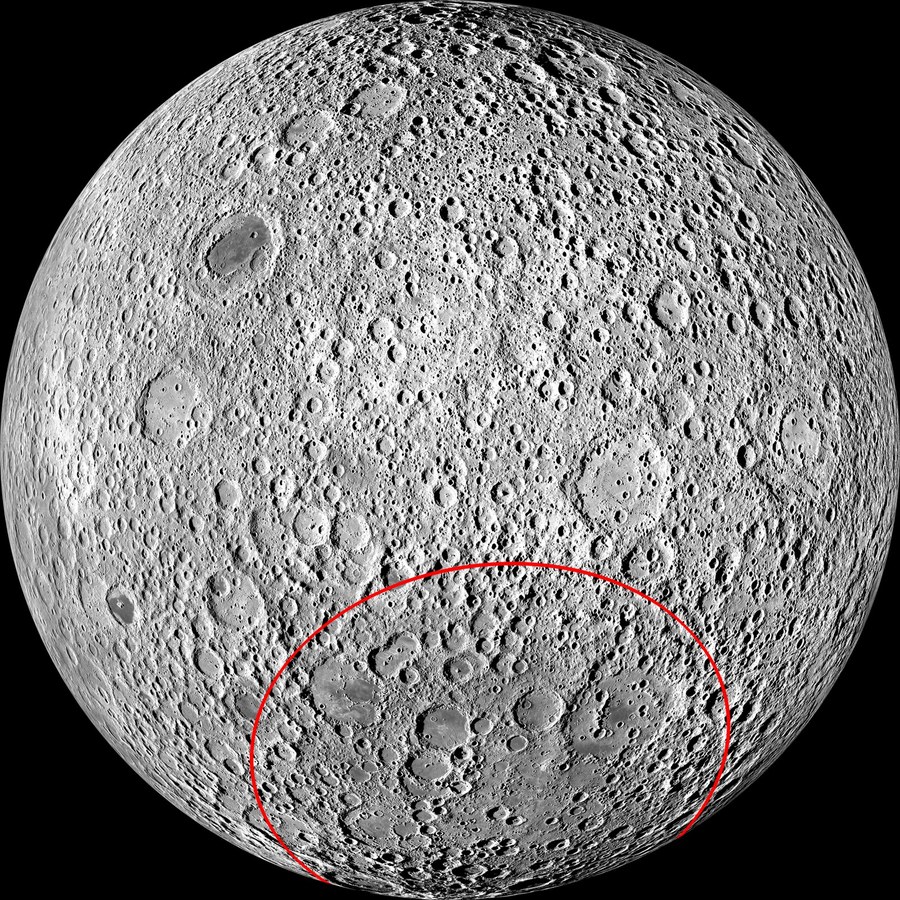
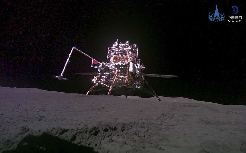
Left: the far side of the Moon, with the South Pole–Aitken basin outlined in red. Image: NASA Lunar Reconnaissance Orbiter (public domain). Right: Chang'e-6 on the far side, photographed by its small rover. Photo: CNSA/Xinhua.
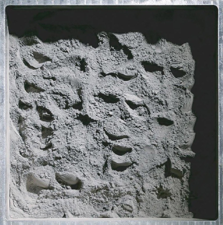
Far-side soil scooped by Chang'e-6, in the laboratory; the bar is 2 cm. Photo: Li and others (2024), National Science Review (CC BY 4.0).
The question. Is the far-side lava older than the youngest lava sampled on the near side, 2030 ± 4 million years (Chang'e-5; Li and others, 2021)? That age is so precise that we treat it as exact.
The method: the bootstrap, because the answer is a difference of two ages, and the bootstrap gives an interval for any number computed from the data. As in Your turn 5: redraw the rows with replacement, fit a line, turn its slope into an age; repeat 10,000 times; keep the middle 95%.
The data. far_side: 59 laser spots on the lava's crystals (Cui and others, 2024);
fragment names the piece of lava each spot is on.
far_side.head()
✏️ Your turn 10
How old is the far-side lava, and how sure is that age?
Why: Your turns 3 and 5 on a new rock.
- The figure: the spots,
parentacross anddaughterup, with the fitted line. far_age: the age, withrb_decay.far_agesandfar_range: 10,000 bootstrap ages (seed 88) and their middle 95%.
Use these names, because the self-check looks for them: far_age, far_ages and far_range.
# ← your answer here: replace every ... with code
far_model = ...  # a line fitted to the spots: parent (as a table) to daughter
b = ...          # b̂: its slope
far_age = ...    # t = ln(1 + b̂) / λ, in millions of years
print("the far-side lava is", round(far_age, 1), "million years old")

plt.figure(figsize=(7, 5))
...  # a scatter plot of far_side: the parent column across, the daughter column up
...  # the fitted line in red: the parent column across, ŷ = â + b̂ × parent up: the line's daughter at each spot's parent
plt.xlabel("parent: rubidium-87 / strontium-86")
plt.ylabel("daughter: strontium-87 / strontium-86")
plt.title(f"Chang'e-6 far-side lava: {len(far_side)} spots")
plt.show()

rng = np.random.default_rng(88)
far_ages = []
for i in range(10000):
    resample = ...        # as many rows as far_side has, drawn with replacement
    resample_model = ...  # a line fitted to them
    b = ...               # b̂: this line's slope
    far_ages.append(...)  # t = ln(1 + b̂) / λ, in millions of years
far_range = ...           # the middle 95% of far_ages
print("bootstrap: 95% interval", far_range.round(1), "million years")
# Self-check: run this after your answer. You do not need to read it — it only says whether something is off.
assert round(far_age, 1) == 2836.1, "fit far_side's parent (double brackets) to its daughter; convert with rb_decay"
assert [round(x, 1) for x in far_range] == [2774.8, 2973.2], "seed 88; sample len(far_side) rows with replacement each time; fit; convert; the 2.5th and 97.5th percentiles"
print(f"✓ Your turn 10 — the far-side lava is {far_age:.0f} million years old; 95% interval {far_range[0]:.0f} to {far_range[1]:.0f}")
What the numbers mean. How do your age and interval compare with the authors' 2839 ± 95 million years?
✏️ Your turn 11
Is the far-side lava older than the near side's?
Why: an interval for a difference, as for the length of the ice age in Your turn 9: subtract the near-side age from every redrawn age.
gap:far_ageminus the near-side age.gap_range: the middle 95% of thefar_agesminus the near-side age.
Use these names, because the self-check looks for them: gap and gap_range.
# ← your answer here: replace every ... with code
near_age = 2030  # million years: the youngest near-side lava, Chang'e-5
gap = ...        # the far-side age minus the near-side age
gap_range = ...  # the middle 95% of each redrawn far-side age minus the near-side age (far_ages is a list: make it an array first)
print("the far side is", round(gap, 1), "million years older; 95% interval", gap_range.round(1))
# Self-check: run this after your answer. You do not need to read it — it only says whether something is off.
assert round(gap, 1) == 806.1, "far_age minus near_age"
assert [round(x, 1) for x in gap_range] == [744.8, 943.2], "np.array(far_ages) minus near_age, then the 2.5th and 97.5th percentiles"
print(f"✓ Your turn 11 — the far side is {gap:.0f} million years older, 95% interval {gap_range[0]:.0f} to {gap_range[1]:.0f}")
What the numbers mean. Is zero inside the interval of the gap, and what does that say about the two sides of the Moon?
Problem 2 (optional): Did large life appear at the same time on two continents? (the formula)
Optional. Your turns 12 and 13 are not graded. Do them if you have time: the same steps date many things.
After the last Snowball Earth ended, about 635 million years ago, the first organisms large enough to see appear in the rocks: soft-bodied fronds and discs, some perhaps early animals. The best-known site is Mistaken Point in Newfoundland, eastern Canada.
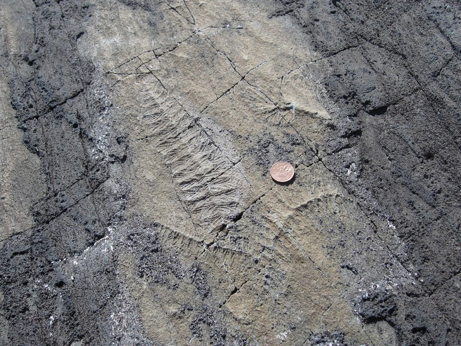
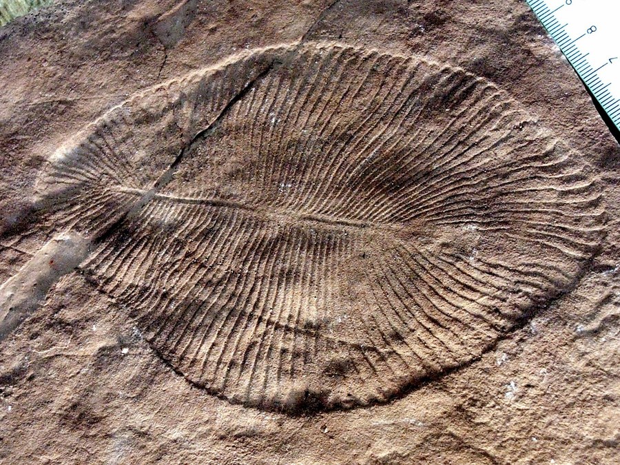
Left: a frond-shaped fossil at Mistaken Point, Newfoundland, with a coin for scale. Photo: Alicejmichel, Wikimedia Commons (CC BY-SA 4.0). Right: Dickinsonia, a later Ediacaran organism. Photo: Verisimilus, Wikimedia Commons (CC BY 2.5).
How do you date a fossil? By a rock layer next to it.
- Newfoundland: volcanic ash about 25 m above the first fronds, 574.17 ± 0.66 million years old by a uranium clock (Matthews and others, 2021). We treat it as exact.
- Yukon, northwest Canada: the same kinds of fossil lie in dark, organic-rich mudstone, which holds the Snowball cap's rhenium-osmium clock. Rooney and others (2020) dated one layer, J1719.
The question. The two places were then on different continents. Did these organisms appear in both at the same time? If so, they were widespread from the start.
The method: the formula, because J1719 has only 8 samples, and with so few the bootstrap's redraws are lumpy (part 3). As in Your turn 6, with $\hat{b}$ the slope, $e_i$ the residuals and $x_i$ the parents:
$$s = \sqrt{\frac{\sum_i e_i^2}{n - 2}}, \qquad S_{xx} = \sum_i (x_i - \bar{x})^2, \qquad \mathrm{SE}(\hat{b}) = \frac{s}{\sqrt{S_{xx}}}, \qquad \hat{b} \pm t_{95}\,\mathrm{SE}(\hat{b})$$
Each end of the slope's interval becomes an age.
The data. fossil_layer: the 8 samples of J1719, parent and daughter as for the
Snowball cap.
fossil_layer
✏️ Your turn 12
How old is layer J1719, and how sure is that age?
Why: Your turns 3 and 6 on a new rock. Each name is a symbol in the math: b is $\hat{b}$, e is $e_i$, s is $s$, Sxx is $S_{xx}$,
SE_b is $\mathrm{SE}(\hat{b})$, t95 is $t_{95}$, and b_ends holds $\hat{b} \pm t_{95}\,\mathrm{SE}(\hat{b})$.
j1719_model,bandj1719_age: a line fitted tofossil_layer, its slope, and its age withre_decay.e,s,Sxx,SE_bandb_ends: the formula's steps, with the givent95; the given last line turns the two ends into ages,j1719_formula_range.
Use these names, because the self-check looks for them: j1719_age and
j1719_formula_range.
# ← your answer here: replace every ... with code
j1719_model = ...  # a line fitted to the layer: parent (as a table) to daughter
b = ...            # b̂: its slope
j1719_age = ...    # t = ln(1 + b̂) / λ with re_decay, in millions of years
print("layer J1719 is", round(j1719_age, 1), "million years old")

e = ...                                                    # e_i = y_i − ŷ_i: each daughter minus the fitted line's daughter at its parent
s = ...                                                    # s = √( Σ e_i² / (n − 2) ), with n = len(e)
Sxx = ...                                                  # S_xx = Σ (x_i − x̄)², with x the parent column of fossil_layer
SE_b = ...                                                 # SE(b̂) = s / √S_xx
t95 = 2.4469                                               # t_95 from the t-table: n − 2 = 6 degrees of freedom
b_ends = ...                                               # b̂ ± t_95 × SE(b̂): the lower and the upper end, as one array
j1719_formula_range = np.log(1 + b_ends) / re_decay / 1e6  # t = ln(1 + b̂) / λ at each end, in millions of years
print("formula: 95% interval", j1719_formula_range.round(1), "million years")
# Self-check: run this after your answer. You do not need to read it — it only says whether something is off.
assert round(j1719_age, 1) == 573.1, "fit fossil_layer's parent (double brackets) to its daughter; convert with re_decay"
assert [round(x, 1) for x in j1719_formula_range] == [570.7, 575.5], "Your turn 6's steps on fossil_layer: e, s, Sxx, SE_b, then b_ends with t95 = 2.4469"
print(f"✓ Your turn 12 — layer J1719 is {j1719_age:.1f} million years old; formula interval {j1719_formula_range[0]:.1f} to {j1719_formula_range[1]:.1f}")
What the numbers mean. How do your age and interval compare with the authors' 574.0 ± 4.7 million years?
✏️ Your turn 13
Did the first large organisms appear at the same time in Canada and in Newfoundland?
Why: the question of Your turn 11, with the formula's interval: subtract the Newfoundland age from the age and from each end of the interval.
fossil_gap:j1719_ageminus the Newfoundland age.fossil_gap_range: each end ofj1719_formula_rangeminus the Newfoundland age.
Use these names, because the self-check looks for them: fossil_gap and fossil_gap_range.
# ← your answer here: replace every ... with code
newfoundland_age = 574.17  # million years: ash above the oldest complex fossils in Newfoundland
fossil_gap = ...           # the J1719 age minus the Newfoundland age
fossil_gap_range = ...     # each end of the formula's interval minus the Newfoundland age
print("Canada minus Newfoundland:", round(fossil_gap, 1), "million years; 95% interval", fossil_gap_range.round(1))
# Self-check: run this after your answer. You do not need to read it — it only says whether something is off.
assert round(fossil_gap, 1) == -1.0, "j1719_age minus newfoundland_age"
assert [round(x, 1) for x in fossil_gap_range] == [-3.4, 1.4], "j1719_formula_range minus newfoundland_age"
print(f"✓ Your turn 13 — Canada minus Newfoundland: {fossil_gap:.1f} million years")
What the numbers mean. Is zero inside your interval? What can you say, and what can you not say, about when the first large organisms appeared in the two places?