Earthquake or nuclear explosion?
EPS 88 · PyEarth. Open your own copy on DataHub: click here.
The Comprehensive Nuclear-Test-Ban Treaty, opened for signature in 1996, bans every nuclear explosion, though it has not yet entered into force. A test can be hidden underground, out of sight, but the ground still shakes, and stations thousands of kilometres away record it. The trouble is that the Earth has thousands of earthquakes a year. To check a ban, you have to pick out the explosions among them, and you have to be right, because a false alarm accuses a country of breaking a treaty.
Today you work with 1,118 real events from the International Seismological Centre's catalogue: 117 nuclear explosions and 1,001 earthquakes in the regions around the test sites. You learn how to score a rule when explosions are rare, how to keep that score honest, how to find a line that separates the two, and where to set the alarm. At the end of class you ask the line about five explosions it has never seen, North Korea's. At home you fit the line in one part of the world and check it in another.
Every place you write something opens with a pencil icon and the words Your turn, and is
followed by a cell that already has the shape of the answer written in, with ... wherever your
code goes. Replace every ..., run every cell so your answers and figures are
saved in the file, then download this notebook itself — the .ipynb file — and upload it
to Gradescope. Not a PDF: the marking reads your notebook, and a PDF cannot be read.
In JupyterLab: File ▸ Download, or right-click the file in the left-hand panel and choose
Download.
Two habits from the first minute. A cell runs when you press Shift+Enter, and the notebook remembers everything it has already run — so when something breaks and you cannot see why, Kernel → Restart Kernel and Run All Cells throws the memory away and rebuilds it from the top. That is never the wrong thing to do.
What you'll be able to do
The science. Say why an explosion and an earthquake of the same size shake the ground differently, and which seismic measurement shows it; and judge a rule that flags explosions by the two mistakes it can make.
The code. Precision, recall and F1 by hand, then with precision_score, recall_score and
f1_score · train_test_split with stratify, into training, validation and test · a grid of
lines scored by counting · LogisticRegression with fit and predict_proba · an alarm level
chosen on validation events and tested once.
Fifteen places where you write something: eleven in class, four at home. Each is headed Your turn.
The six questions of the class:
- How could a seismometer tell a test from an earthquake?
- How do we score a rule when explosions are rare?
- How do we keep the score honest?
- Can one line through mb and Ms split them?
- Where should the alarm go?
- Does the line work somewhere new?
Setup
Run the next cell once. It reads the events, stored with the course: every event in three regions
with test sites, plus North Korea, for which the International Seismological Centre (ISC) Bulletin
lists both magnitudes this week uses. It splits off the five North Korean explosions into their own
table, korea, for the end of class, and keeps the rest in events. It also reads the coastlines
for the map, and makes grid, a table of points spread over the mb–Ms plane, for the probability
map at the end of class, over the same mb and Ms range, 2 to 7, as the treaty's screening plot.
import numpy as np
from sklearn.linear_model import LogisticRegression
from sklearn.model_selection import train_test_split
from sklearn.metrics import accuracy_score, precision_score, recall_score, f1_score
from sklearn.metrics import confusion_matrix, roc_auc_score
import pandas as pd
import matplotlib.pyplot as plt

# house style, set once, so every plot cell below holds only what matters
plt.rcParams.update({"figure.dpi": 110,
                     "axes.grid": True, "grid.alpha": 0.3, "axes.axisbelow": True})

CACHE = "https://raw.githubusercontent.com/AI4EPS/EPS88_PyEarth/main/data"

# One row per event: when and where, its two magnitudes, and what it was.
# Source: International Seismological Centre (2026), On-line Bulletin, https://doi.org/10.31905/D808B830
table = pd.read_csv(CACHE + "/week09_mb_ms_isc.csv")
events = table[table["region"] != "Korea"]                           # the class's events
korea = table[(table["region"] == "Korea") & table["is_explosion"]]  # North Korea's explosions, kept apart
coast = pd.read_csv(CACHE + "/coastlines.csv")

# the grid: every pair of mb and Ms from 2 to 7, in steps of 0.05, for the map
grid_mb = []
grid_Ms = []
for mb in np.arange(2, 7.01, 0.05):
    for Ms in np.arange(2, 7.01, 0.05):
        grid_mb.append(mb)
        grid_Ms.append(Ms)
grid = pd.DataFrame({"mb": grid_mb, "Ms": grid_Ms})
print(len(events), "events:", events["is_explosion"].sum(), "explosions and", (events["is_explosion"] == False).sum(), "earthquakes")
1. How could a seismometer tell a test from an earthquake?
An underground test. A nuclear device is placed hundreds of metres underground, at the bottom of a drilled shaft or at the end of a tunnel dug into a mountain, sealed in, and fired. Usually nothing reaches the surface but the shaking (and sometimes radioactive gas that seeps out), and later, often, a crater where the rock above the blast collapses. (Firing a device inside a large underground cavity can muffle the shaking many times over, one reason small tests are hard to find.)
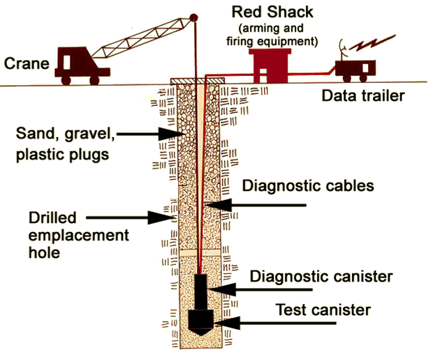
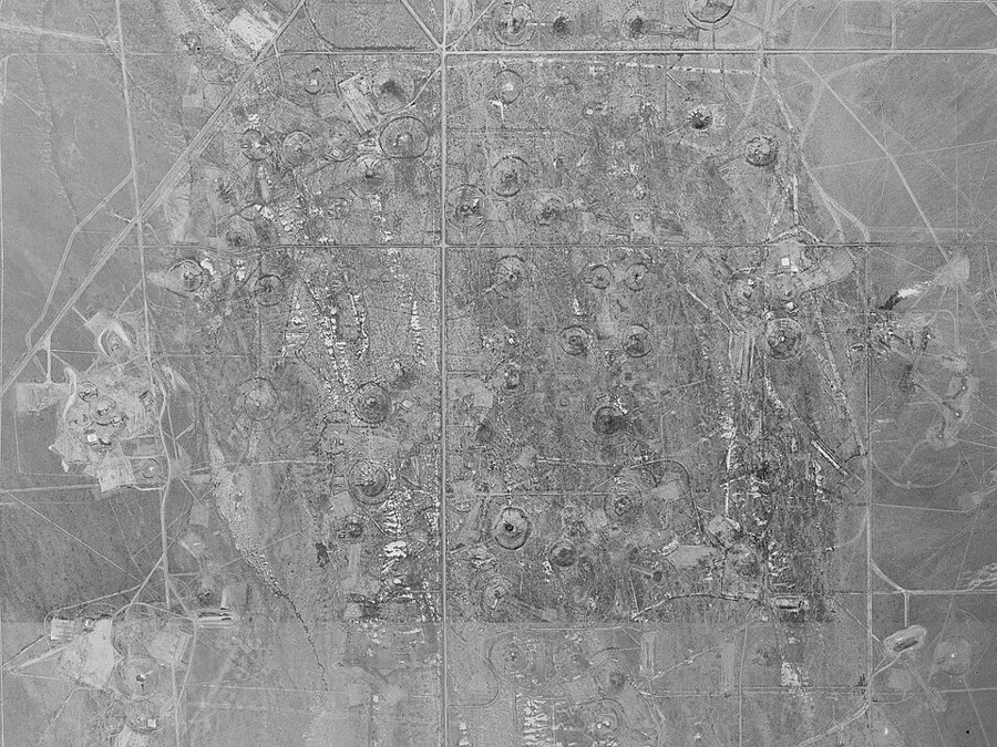
Left: a vertical underground test at the Nevada Test Site, the device at the bottom of a drilled hole. Diagram: US Government (public domain). Right: craters left at the Nevada Test Site where the ground collapsed into the cavities of underground tests. Photo: USGS (public domain). Both via Wikimedia Commons.
Two sizes for one event. Shaking travels as waves. The fastest, the P waves, push and pull the rock along their path; S waves shake it from side to side; and the slow surface waves roll along the ground behind them.
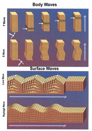
How each kind of seismic wave moves the ground: two body waves (P and S) and two surface waves (Love and Rayleigh). Figure: USGS (public domain), via Wikimedia Commons.
An explosion pushes the rock outward from one small spot, the same in every direction, so most of its shaking leaves as P waves. An earthquake is two blocks of rock slipping past each other along a fault: it sends out strong S waves, and, because the slip spreads over a large patch of fault and lasts longer, strong surface waves too.
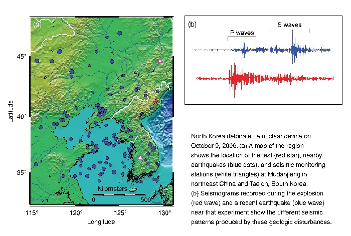
North Korea's first test, 9 October 2006. Left: the test site (red star), earthquakes nearby (blue dots) and two seismic stations (triangles). Right: the explosion (red) and a recent earthquake nearby (blue) recorded at a station: the explosion's shaking is mostly P waves; the earthquake's largest shaking is its S waves. Figure: Lawrence Livermore National Laboratory, Science & Technology Review (March 2009), via the Berkeley Seismological Laboratory blog.
So seismologists give each event two sizes. The body-wave magnitude mb is read from the first, fast P wave. The surface-wave magnitude Ms is read from the slow surface waves that follow. A small, sudden source like an explosion puts little energy into those long surface waves, so for its mb, an explosion has a small Ms. That one sentence is the physics of the whole week; the rest is how to use it well.
events[["date", "region", "depth", "mb", "Ms", "is_explosion"]].head()
Each row is one event: its date, its region, its depth below the surface in km, its two
magnitudes, and is_explosion, the label: True for a nuclear explosion, False for an
earthquake. The events come from three regions with test sites, from 1970 to 1996:
- the western US: 405 events, 36 of them explosions, 35 at the Nevada Test Site and one in Colorado;
- Central Asia: 696 events, 64 explosions, 53 at the Soviet test site near Semipalatinsk (now in Kazakhstan) and 11 at China's Lop Nur;
- Novaya Zemlya, an Arctic island where the Soviet Union also tested: 17 events, all explosions.
Only events with both magnitudes are kept. Small explosions often have no Ms at all, so the table holds mostly large ones: only 9 of its 117 explosions have an mb below 5.4. Keep that in mind when the line meets smaller ones.
explosions = events[events["is_explosion"]]
earthquakes = events[events["is_explosion"] == False]

plt.figure(figsize=(10, 4.5))
plt.plot(coast["lon"], coast["lat"], color="0.6", lw=0.5)
plt.scatter(earthquakes["lon"], earthquakes["lat"], s=6, color="tab:blue", label="earthquake")
plt.scatter(explosions["lon"], explosions["lat"], s=30, marker="*", color="red", label="nuclear explosion")
plt.xlim(-180, 180)
plt.ylim(0, 90)
plt.gca().set_aspect("equal")
plt.xlabel("longitude (degrees east)")
plt.ylabel("latitude (degrees north)")
plt.title("The events of the table")
plt.legend(loc="lower left")
plt.show()
2. How do we score a rule when explosions are rare?
This is classification. In the regression weeks a model answered with a number. Here it answers with a label: explosion or earthquake. A guess is a column of True and False, one per event, from a rule or a model. It is scored against the label.
The laziest rule is to say "earthquake" every time. It is the baseline, the simplest rule there is, scored first: a rule that cannot beat it does no useful work.
✏️ Your turn 1
How good is "always earthquake"?
Why: a score is only useful if a rule that does no work scores badly. Find out what the usual score, accuracy, gives the laziest rule.
always_earthquake: a guess of False for every event, given. It is written as a mask on a column (no event has an mb above 100) so that it is a column of True and False like every other guess this week.accuracy: the share of events where the guess equals the label: the mean of the maskalways_earthquake == events["is_explosion"]. The next line printsaccuracy_scorebeside it.found: how many explosions the rule flags: the sum of the maskalways_earthquake & events["is_explosion"].
Use these names, because the self-check looks for them: accuracy and found.
# ← your answer here: replace every ... with code
always_earthquake = events["mb"] > 100  # False for every event
accuracy = (... == ...).mean()          # the guess, and the label
print("accuracy by hand:", round(accuracy, 3), "  with accuracy_score:", round(accuracy_score(events["is_explosion"], always_earthquake), 3))
found = (... & ...).sum()               # flagged, and an explosion
print("explosions flagged:", found, "of", events["is_explosion"].sum())
# Self-check: run this after your answer. You do not need to read it — it only says whether something is off.
assert round(accuracy, 3) == 0.895, "the mean of the mask always_earthquake == events['is_explosion']"
assert found == 0, "the sum of always_earthquake & events['is_explosion']"
print(f"✓ Your turn 1 — 'always earthquake' scores {accuracy:.3f} and finds {found} explosions")
Accuracy 0.895, and not one explosion found. Nine events in ten are earthquakes, so a rule that never flags is right nine times in ten. When one label is rare, accuracy hides the misses. A treaty needs scores that count the two kinds of mistake apart.
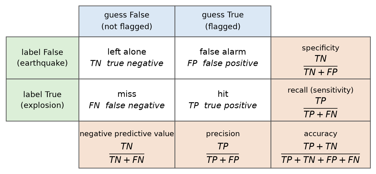
Four counts. Sort the events by label and by guess into four groups. A hit is an explosion the rule flagged, a miss an explosion it did not flag, and a false alarm an earthquake it flagged. The fourth group, earthquakes the rule leaves alone, is the right answer for most events. Two scores come from the counts:
- precision = hits / (hits + false alarms): of the events you flagged, the share that were explosions;
- recall = hits / (hits + misses): of the explosions, the share you flagged.
F1 joins them into one number, $F_1 = 2PR/(P+R)$ with $P$ the precision and $R$ the recall, which is high only when both are high.
Ten made-up events, two of them explosions, and the rule "flag every event with mb 5.7 or more":
ten_events = pd.DataFrame({"mb": [4.2, 4.5, 4.8, 5.0, 5.1, 5.3, 5.6, 5.8, 5.9, 6.2],
                           "is_explosion": [False, False, False, False, False, True, False, False, True, False]})
ten_events["flagged"] = ten_events["mb"] >= 5.7
print(ten_events)
print("confusion_matrix:")
print(confusion_matrix(ten_events["is_explosion"], ten_events["flagged"]))
Count by eye: the rule flags the three events with mb 5.8, 5.9 and 6.2. One of them, 5.9, is an explosion: 1 hit and 2 false alarms. The explosion with mb 5.3 is missed. The six other earthquakes are left alone. So precision is 1 / (1 + 2) = 1/3, recall 1 / (1 + 1) = 1/2, and F1 = 2 × 1/3 × 1/2 / (1/3 + 1/2) = 0.4.
confusion_matrix prints the same four counts as a table of 2 by 2: rows are the label (False,
then True), columns the guess (False, then True). The names you will meet in other courses and
papers: a hit is a true positive (TP), a false alarm a false positive (FP), a miss a false
negative (FN), and an earthquake left alone a true negative (TN). Each score is read off one row
or one column:
✏️ Your turn 2
How well does a cut on mb alone find the explosions?
Why: the simplest rule that looks at the data is a cut on one column. Scoring it uses all three new scores, which you compute from the counts yourself.
guess_mb: True where an event's mb is 5.7 or more.hits,misses,false_alarms: the three counts, each as the sum of a mask. (guess_mb == Falseis the mask of the events not flagged.)precision_mb,recall_mb,f1_mb: the three scores from your counts, by the formulas above. The line after them prints whatprecision_score,recall_scoreandf1_scoregive for the same label and guess.- The figure: histograms of mb for the earthquakes and the explosions, with a line at the cut.
Use these names, because the self-check looks for them: hits, misses, false_alarms,
precision_mb, recall_mb and f1_mb.
# ← your answer here: replace every ... with code
label = events["is_explosion"]
guess_mb = events["mb"] >= ...                    # the cut
hits = (... & ...).sum()                          # flagged, and an explosion
misses = ((guess_mb == False) & ...).sum()        # not flagged, and an explosion
false_alarms = (guess_mb & (... == False)).sum()  # flagged, and an earthquake
precision_mb = ...                                # of the flagged events, the share that are explosions
recall_mb = ...                                   # of the explosions, the share flagged
f1_mb = ...                                       # 2PR / (P + R)
print(hits, "hits,", misses, "misses,", false_alarms, "false alarms")
print("by hand:      precision", round(precision_mb, 3), " recall", round(recall_mb, 3), " F1", round(f1_mb, 3))
print("scikit-learn: precision", round(precision_score(label, guess_mb), 3), " recall", round(recall_score(label, guess_mb), 3), " F1", round(f1_score(label, guess_mb), 3))

plt.figure(figsize=(8, 4))
bins = np.arange(3.65, 7.05, 0.1)                                     # one bin per tenth of a magnitude, the same for both
plt.hist(..., bins=bins, alpha=0.6, label="earthquakes")              # the earthquakes' mb
plt.hist(..., bins=bins, alpha=0.6, color="red", label="explosions")  # the explosions' mb
plt.axvline(..., color="black", label="the cut")                      # the cut
plt.xlabel("body-wave magnitude mb")
plt.ylabel("number of events")
plt.title("mb alone: the two labels overlap")
plt.legend()
plt.show()
# Self-check: run this after your answer. You do not need to read it — it only says whether something is off.
assert (hits, misses, false_alarms) == (85, 32, 105), "a hit is guess & label; a miss (guess == False) & label; a false alarm guess & (label == False)"
assert round(precision_mb, 3) == 0.447, "precision is hits / (hits + false_alarms)"
assert round(recall_mb, 3) == 0.726, "recall is hits / (hits + misses)"
assert round(f1_mb, 3) == 0.554, "F1 is 2 * precision_mb * recall_mb / (precision_mb + recall_mb)"
print(f"✓ Your turn 2 — the cut on mb: {hits} hits, {misses} misses, {false_alarms} false alarms, F1 {f1_mb:.3f}")
The cut finds 85 of 117 explosions, but it also flags
105 earthquakes: precision 0.447, recall 0.726, F1
0.554. The histogram shows why no cut on mb can do much better: big earthquakes and big
explosions have the same mb. From here on the notebook calls f1_score, which does exactly the
arithmetic you just did. A cut on Ms alone is worse:
guess_ms = events["Ms"] <= 4.9     # flag events with small surface waves; 4.9 is about the best cut on Ms
print("Ms of 4.9 or less: F1", round(f1_score(label, guess_ms), 3))
F1 0.231. Each magnitude alone fails, because in each one the two labels overlap. Part 4 puts them together. First, two rules that keep every score in this notebook honest.
3. How do we keep the score honest?
Rule one: no column may already know the answer. Depth looks tempting: earthquakes start kilometres down, and a test hole is a few hundred metres deep.
✏️ Your turn 3
How well does "depth is 0" find the explosions, and why?
Why: a rule that scores almost perfectly deserves the hardest look.
guess_depth: True where an event'sdepthis exactly 0.f1_depth: its F1.explosions_at_0andearthquakes_at_0: how many explosions, and how many earthquakes, have a depth of exactly 0.
Use these names, because the self-check looks for them: f1_depth, explosions_at_0 and
earthquakes_at_0.
# ← your answer here: replace every ... with code
guess_depth = events["depth"] == ...  # a depth of exactly 0
f1_depth = f1_score(..., ...)         # the label, then the depth guess
explosions_at_0 = (... & ...).sum()   # depth 0, and an explosion
earthquakes_at_0 = (... & ...).sum()  # depth 0, and an earthquake
print("depth is 0: F1", round(f1_depth, 3))
print("explosions at depth 0:", explosions_at_0, "of", label.sum(), "  earthquakes at depth 0:", earthquakes_at_0)
# Self-check: run this after your answer. You do not need to read it — it only says whether something is off.
assert round(f1_depth, 3) == 0.996, "guess_depth is events['depth'] == 0; then f1_score"
assert (explosions_at_0, earthquakes_at_0) == (117, 1), "the sums of guess_depth & label and guess_depth & (label == False)"
print(f"✓ Your turn 3 — 'depth is 0' scores F1 {f1_depth:.3f}: {explosions_at_0} explosions and {earthquakes_at_0} earthquake at depth 0")
An F1 of 0.996, nearly perfect, and useless. All 117 explosions have depth 0.0, and the catalogue marks each of those depths as fixed by the analyst, not measured from the waves: the analyst set it to 0 because the event was already known to be an explosion. The column knew the answer before anyone looked. This is called leakage: a column that already holds the answer. When a score looks too good, first ask whether a column already knew the answer. (Shallow depths are hard to measure, so the catalogue fixed the depth of 343 earthquakes too, and depth cannot separate two shallow events.)
Rule two: training, validation and test. You met this in the model-selection week. Every rule from here on has something to choose: a gap, a slope, an alarm level. Anything chosen by looking at events will score well on those events, so the events that judge the choice must be kept apart:
- the training events, used to fit and to search;
- the validation events, used to choose between the rules found on training;
- the test events, used once, at the end, to report how well the chosen rule does.
train_test_split cuts the rows at random. Explosions are only one event in ten, so a random cut
can leave a part with too few; stratify= the label keeps the share of explosions the same in
every part. Two cuts make the three parts: first 20 percent off for the test, then 25 percent of
the rest for validation.
✏️ Your turn 4
How do the events divide into training, validation and test?
Why: every choice in the rest of the class is made on training or validation events, and the test events are opened once, at the end.
rest,test:train_test_splitofevents, 20 percent to the test, stratified on the label,random_state=42.train,validation:train_test_splitofrest, 25 percent to validation, stratified onrest's label,random_state=42.- The print that counts the events and explosions in each part is given.
Use these names, because the self-check looks for them: train, validation and test.
# ← your answer here: replace every ... with code
rest, test = train_test_split(..., test_size=..., random_state=42, stratify=...)  # every event; the test's share; their label
train, validation = train_test_split(..., test_size=..., random_state=42, stratify=...)  # the rest; validation's share of it; its label
for name, part in [("training", train), ("validation", validation), ("test", test)]:
    print(name, ":", len(part), "events,", part["is_explosion"].sum(), "explosions")
# Self-check: run this after your answer. You do not need to read it — it only says whether something is off.
assert (len(train), len(validation), len(test)) == (670, 224, 224), "20 percent of events to test, then 25 percent of the rest to validation"
assert (train["is_explosion"].sum(), validation["is_explosion"].sum(), test["is_explosion"].sum()) == (70, 24, 23), "stratify each cut on its table's is_explosion"
print(f"✓ Your turn 4 — {len(train)} training, {len(validation)} validation and {len(test)} test events")
670 training events (70 explosions), 224 for
validation (24) and 224 for the test (23).
Without stratify, the number of explosions that lands in the test part depends on the luck of
the cut:
for seed in [0, 1, 2, 3, 4]:
    rest_plain, test_plain = train_test_split(events, test_size=0.2, random_state=seed)   # no stratify
    print("random_state", seed, ": the test part gets", test_plain["is_explosion"].sum(), "explosions")
Anywhere from 21 to 26 explosions: with so few, a test score would move with the cut as much as with the rule. Stratified, it is 23 every time.
4. Can one line through mb and Ms split them?
Recall the physics: for its mb, an explosion has a small Ms. Plot the training events in the two magnitudes together:
train_explosions = train[train["is_explosion"]]
train_earthquakes = train[train["is_explosion"] == False]

plt.figure(figsize=(6.5, 5.5))
plt.scatter(train_earthquakes["mb"], train_earthquakes["Ms"], s=8, color="tab:blue", alpha=0.5, label="earthquake")
plt.scatter(train_explosions["mb"], train_explosions["Ms"], s=14, color="red", alpha=0.7, label="explosion")
plt.plot([2, 7], [2, 7], color="0.4", label="Ms = mb")
plt.xlim(2, 7)
plt.ylim(2, 7)
plt.gca().set_aspect("equal")     # the same frame as the treaty's screening plot, so the two compare
plt.xlabel("body-wave magnitude mb")
plt.ylabel("surface-wave magnitude Ms")
plt.title("The training events, in two magnitudes")
plt.legend()
plt.show()
The two labels, which overlapped in each magnitude alone, come apart in the two together: the explosions sit below the earthquakes. A line below Ms = mb could split them: flag an event when Ms < mb − gap. Magnitudes have one decimal, so many events would sit exactly on a gap like 1.0; gaps that end in 5 avoid that: 0.55, 0.75, 0.95, 1.15, 1.35.
✏️ Your turn 5
Which gap draws the best line, on the training events?
Why: the simplest line has one number to choose. Trying each and keeping the best is the search that every fitting method does, in its plainest form.
- The loop, which you write yourself. For each gap in
gaps: the guess, True where a training event's Ms is below its mb minus the gap; its F1 against the training label; and a print of the gap and the F1. Each comment in the cell is one line for you to write. gap: the gap with the best F1, read from your printout.
Use these names, because the self-check looks for them: gap and f1_gap.
# ← your answer here: replace every ... with code
gaps = [0.55, 0.75, 0.95, 1.15, 1.35]
# for each gap in gaps:
#     guess: True where train["Ms"] is below train["mb"] minus the gap
#     f1_gap: the F1 of that guess, the training label first
#     print the gap and round(f1_gap, 3)
...

gap = ...  # the gap with the best F1 in your printout
f1_gap = f1_score(train["is_explosion"], train["Ms"] < train["mb"] - gap)
print("chosen gap", gap, ": training F1", round(f1_gap, 3))
# Self-check: run this after your answer. You do not need to read it — it only says whether something is off.
assert gap == 0.95 and round(f1_gap, 3) == 0.826, "of the five gaps, 0.95 gives the best training F1"
print(f"✓ Your turn 5 — the line by eye: gap {gap}, training F1 {f1_gap:.3f}")
The loop printed 0.496, 0.694, 0.826, 0.815, 0.621: gap 0.95 is best, F1 0.826 on the training events. But this line's slope was fixed at 1. A line has two numbers, a slope and an offset: flag an event when Ms < slope × mb − offset. The same search, over both numbers at once, is a grid, as in the week you fitted the Hubble line: every slope with every offset, each line scored, the best kept.
✏️ Your turn 6
Which line, of 560, separates the training events best?
Why: this is what fitting does: try lines and keep the one that scores best. Here you do it by counting, with F1 as the score.
- The two loops: for each offset in
offsets, for each slope inslopes, the guess, True where a training event's Ms is below slope × mb − offset, and its F1, appended tof1s. best_f1,best_slope,best_offset: inside the loop, when a line beats the best so far, keep its F1, slope and offset (anif, as in week 2). Ties keep the first line found.- The picture of every F1, slope across and offset up, is given.
Use these names, because the self-check looks for them: f1s, best_f1, best_slope and
best_offset.
# ← your answer here: replace every ... with code
slopes = np.arange(0.75, 2.5, 0.25).round(2)                  # slopes from 0.75 to 2.25, in steps of 0.25
offsets = np.arange(0.05, 8.0, 0.1).round(2)                  # offsets that end in 5, from 0.05 to 7.95
f1s = []
best_f1 = 0
for offset in offsets:
    for slope in slopes:
        guess = train["Ms"] < ... * train["mb"] - ...         # this line
        f1_line = f1_score(..., ...)                          # the training label, then this guess
        f1s.append(f1_line)
        if f1_line > ...:                                     # better than the best so far
            best_f1, best_slope, best_offset = ..., ..., ...  # keep this line's F1, slope and offset
print(len(f1s), "lines tried; the best: Ms <", best_slope, "x mb -", best_offset, ", training F1", round(best_f1, 3))

f1_grid = np.array(f1s).reshape(len(offsets), len(slopes))  # the same numbers as a grid: one row per offset
plt.figure(figsize=(6, 5))
plt.imshow(f1_grid, extent=[0.625, 2.375, 0, 8], origin="lower", aspect="auto", cmap="viridis")
plt.colorbar(label="training F1")
plt.scatter(best_slope, best_offset, color="red", marker="x", s=80, label="the best line")
plt.xlabel("slope")
plt.ylabel("offset")
plt.title("F1 of every line Ms < slope x mb - offset")
plt.legend(loc="lower right")
plt.show()
# Self-check: run this after your answer. You do not need to read it — it only says whether something is off.
assert round(f1s[71], 3) == 0.851, "for each pair: guess = train['Ms'] < slope * train['mb'] - offset; its F1 against the training label"
assert round(best_f1, 3) == 0.931 and (best_slope, best_offset) == (1.75, 5.25), "keep a line when its F1 beats best_f1"
print(f"✓ Your turn 6 — the grid's best line: Ms < {best_slope} x mb - {best_offset}, training F1 {best_f1:.3f}")
Of 560 lines, the best is Ms < 1.75 × mb − 5.25, training F1 0.931, against 0.826 for the line with slope 1. The bright band in the picture is a ridge of good lines: a steeper slope needs a larger offset. The data chose a slope well above 1.
Logistic regression searches for the same kind of line, but in a different way, and it gives
something the grid cannot: a probability for every event. It works out a value $z$ from the
columns, as LinearRegression did, and bends $z$ into a probability with the S-curve
$$p = \frac{1}{1 + e^{-z}}, \qquad z = a \times \text{mb} + b \times \text{Ms} + c$$
where $p$ is the probability that the event is an explosion, $a$, $b$, $c$ are the three numbers
fit finds, and $e \approx 2.718$. For $z = -2$, $p = 0.12$; for $z = 0$, $p = 0.5$; for $z = 2$,
$p = 0.88$. The events where $z = 0$, so $p = 0.5$, lie on a straight line, the decision
boundary: solved for Ms it is Ms = −(a × mb + c) / b. On one side the model says explosion, on
the other earthquake.
Six made-up events with one number each, the first three earthquakes and the last three explosions, show the S-curve:
six_events = pd.DataFrame({"size": [1, 2, 3, 4, 5, 6],
                           "is_explosion": [False, False, False, True, True, True]})
six_model = LogisticRegression().fit(six_events[["size"]], six_events["is_explosion"])
six_events["probability"] = six_model.predict_proba(six_events[["size"]])[:, 1].round(2)
print(six_events)

sizes = pd.DataFrame({"size": np.arange(0, 7.05, 0.05)})     # sizes from 0 to 7, for drawing the curve
plt.figure(figsize=(6, 3.5))
plt.plot(sizes["size"], six_model.predict_proba(sizes)[:, 1], color="black")
plt.scatter(six_events["size"], six_events["is_explosion"], color="red")
plt.axhline(0.5, color="0.6")
plt.xlabel("size")
plt.ylabel("probability of an explosion")
plt.title("The S-curve on six made-up events")
plt.show()
The probabilities rise from 0.06 to 0.94, and the curve crosses 0.5 halfway between
the last earthquake and the first explosion. predict_proba(...)[:, 1] gives the probability of
True, an explosion, for each row.
How fit scores a curve. Your grid scored a line by counting right and wrong. fit scores a
curve by the probability it gives each event for the label it really has: $p$ for an explosion,
$1 - p$ for an earthquake. Multiplied over all the events, that is the chance the curve gives to
the labels coming out as they did; fit keeps the curve that makes it largest. Against the same
curve moved one unit to the right:
w = six_model.coef_[0][0]      # the number fit found for size
c = six_model.intercept_[0]    # and the constant
size = six_events["size"]
six_label = six_events["is_explosion"]

for name, z in [("fitted curve", w * size + c), ("curve moved right by 1", w * (size - 1) + c)]:
    p = 1 / (1 + np.exp(-z))                          # the S-curve
    own = six_label * p + (1 - six_label) * (1 - p)   # p for an explosion, 1 - p for an earthquake
    chance = 1
    for q in own:
        chance = chance * q                           # multiply the six together
    print(name, ": probability of each event's own label", list(own.round(2)), " all six:", round(chance, 3))
The chance of all six falls from 0.256 to 0.152 when the curve moves: the fitted curve
scores higher. (On six events this cleanly split, an ever steeper curve would score higher still;
fit stops that by keeping the numbers small.) With two columns, fit does the same with $a$,
$b$ and $c$.
✏️ Your turn 7
Does fit find the grid's line, and which line does best on the validation events?
Why: the grid searched by counting, fit by probability. If they agree, you know what fit
did. The validation events, which none of the three lines saw, judge between them.
model:LogisticRegression().fit(...)on the training events:mbandMs, then the label.boundary_slopeandboundary_offset: the boundary written as a line, like the grid's.a, b = model.coef_[0]andc = model.intercept_[0]are given: here a = 5.91, b = -3.31, c = -18.16. The boundary is where z = 0, so a × mb + b × Ms + c = 0. Move a × mb + c to the other side: b × Ms = −a × mb − c. Divide by b: Ms = (−a / b) × mb − c / b. So the slope is −a / b and the offset is c / b. And b is negative: a larger Ms makes an earthquake more likely. Dividing by a negative number turns > into <, so the side where z > 0, the explosions, is Ms < slope × mb − offset, the same form as the grid's line.f1_val_model: the model's F1 on the validation events, withmodel.predict(...). The F1s of the line by eye and the grid's line on the same events are given.
Use these names, because the self-check looks for them: boundary_slope, boundary_offset
and f1_val_model.
# ← your answer here: replace every ... with code
model = LogisticRegression().fit(..., ...)  # the training events: the mb and Ms columns, then the label
a, b = model.coef_[0]                       # the numbers fit found for mb and Ms
c = model.intercept_[0]                     # and the constant
boundary_slope = ...                        # the boundary's slope
boundary_offset = ...                       # the boundary's offset
print("fit's boundary:  Ms <", round(boundary_slope, 2), "x mb -", round(boundary_offset, 2))
print("the grid's line: Ms <", best_slope, "x mb -", best_offset)

val_label = validation["is_explosion"]
f1_val_model = f1_score(val_label, model.predict(...))  # the validation events' two magnitudes
f1_val_eye = f1_score(val_label, validation["Ms"] < validation["mb"] - gap)
f1_val_grid = f1_score(val_label, validation["Ms"] < best_slope * validation["mb"] - best_offset)
print("validation F1:  line by eye", round(f1_val_eye, 3), "  grid's line", round(f1_val_grid, 3), "  logistic regression", round(f1_val_model, 3))
# Self-check: run this after your answer. You do not need to read it — it only says whether something is off.
assert round(boundary_slope, 2) == 1.78 and round(boundary_offset, 2) == 5.48, "slope -a / b, offset c / b, from a model fitted on train"
assert round(f1_val_model, 3) == 0.857, "model.predict on validation[['mb', 'Ms']], scored against validation's label"
print(f"✓ Your turn 7 — fit's boundary Ms < {boundary_slope:.2f} x mb - {boundary_offset:.2f}; validation F1 {f1_val_model:.3f}")
fit lands next to the grid: Ms < 1.78 × mb − 5.48, against the grid's
1.75 and 5.25. Two different ways of searching found nearly the same
line. On the validation events the two tie, F1 0.857 and 0.857, and both beat
the line by eye (0.792): the slope of 1 was too shallow.
So why use logistic regression, if counting finds the line? Because it gives each event a probability, and the last question of the class needs one.
val_explosions = validation[validation["is_explosion"]]
val_earthquakes = validation[validation["is_explosion"] == False]
mb_ends = np.array([2, 7])     # across the whole frame

plt.figure(figsize=(6.5, 5.5))
plt.scatter(val_earthquakes["mb"], val_earthquakes["Ms"], s=10, color="tab:blue", label="earthquake")
plt.scatter(val_explosions["mb"], val_explosions["Ms"], s=18, color="red", label="explosion")
plt.plot(mb_ends, boundary_slope * mb_ends - boundary_offset, color="black", label="fit's boundary")
plt.plot(mb_ends, best_slope * mb_ends - best_offset, color="tab:green", ls=":", label="the grid's line")
plt.plot(mb_ends, mb_ends - gap, color="black", ls="--", label="line by eye")
plt.xlim(2, 7)
plt.ylim(2, 7)
plt.gca().set_aspect("equal")
plt.xlabel("body-wave magnitude mb")
plt.ylabel("surface-wave magnitude Ms")
plt.title(f"Three lines from the training events, on the {len(validation)} validation events")
plt.legend()
plt.show()
5. Where should the alarm go?
predict flags an event when its probability is 0.5 or more. Nothing says 0.5 is right. A missed
explosion is a secret test that got through; a false alarm accuses a state that did nothing, though
an inspection team can check a flagged event by other means. The alarm level is that choice: the
probability at or above which you flag an event. Lower it and you miss fewer explosions but accuse
more earthquakes. It is a choice, so it is made on the validation events.
First, the probability itself, from the three numbers fit found.
✏️ Your turn 8
What probability does the model give each validation event?
Why: predict_proba is the S-curve applied to z. Compute it yourself once, and check.
z: a × mb + b × Ms + c for every validation event, with thea,bandcof Your turn 7.prob_val: the S-curve ofz, 1 / (1 + e^(−z)), withnp.exp.- The next line prints the largest difference from
model.predict_proba(...)[:, 1].
Use these names, because the self-check looks for them: z and prob_val.
# ← your answer here: replace every ... with code
z = ...         # a times mb, plus b times Ms, plus c, for the validation events
prob_val = ...  # the S-curve of z
print("largest difference from predict_proba:", np.max(np.abs(prob_val - model.predict_proba(validation[["mb", "Ms"]])[:, 1])))
# Self-check: run this after your answer. You do not need to read it — it only says whether something is off.
assert np.max(np.abs(prob_val - model.predict_proba(validation[["mb", "Ms"]])[:, 1])) < 1e-9, "z = a * mb + b * Ms + c on validation; then 1 / (1 + np.exp(-z))"
print(f"✓ Your turn 8 — your probabilities match predict_proba")
The difference is at the level of the computer's rounding: predict_proba is exactly this
arithmetic. Now try alarm levels on the same validation events.
✏️ Your turn 9
Which alarm level works best on the validation events?
Why: every level makes its own trade between misses and false alarms. Count both at each level and choose, before the test events are opened.
- The loop: for each level in
levels, flag the validation events whoseprob_valis at or above it; print the level, the hits, the false alarms and the F1; append the F1 tolevel_f1s. chosen_level: the level with the best F1, read from your printout.
Use these names, because the self-check looks for them: level_f1s and chosen_level.
# ← your answer here: replace every ... with code
levels = [0.9, 0.7, 0.5, 0.3, 0.2, 0.1, 0.05]
level_f1s = []
for level in levels:
    flagged = ...          # validation events at or above this level
    hits_v = ...           # flagged, and an explosion
    false_alarms_v = ...   # flagged, and an earthquake
    level_f1s.append(...)  # the F1 at this level
    print("level", level, ":", hits_v, "of", val_label.sum(), "explosions,", false_alarms_v, "false alarms, F1", round(level_f1s[-1], 3))

chosen_level = ...  # the level with the best F1 in your printout
# Self-check: run this after your answer. You do not need to read it — it only says whether something is off.
assert [round(x, 3) for x in level_f1s] == [0.4, 0.769, 0.857, 0.958, 0.939, 0.793, 0.552], "flagged = prob_val >= level; F1 against val_label"
assert chosen_level == 0.3, "the level with the largest F1"
print(f"✓ Your turn 9 — the alarm level chosen on validation: {chosen_level}")
At 0.5 the model flags 18 of 24 validation explosions and no earthquake; at 0.3, 23 explosions for 1 false alarm, F1 0.958, the best. Below that the false alarms grow fast. 0.3 is the level.
Each level is one trade, one point. The ROC curve draws them all at once: the share of explosions caught (up) against the share of earthquakes falsely flagged (across), one point per level. A rule that flagged events at random would catch the same share of each, on the diagonal, the coin toss; the closer the curve hugs the top left, the better the model orders the events.
hit_shares = []
false_alarm_shares = []
for level in [1.0] + levels + [0.0]:     # your levels, and the two ends: flag nothing, flag everything
    flagged = prob_val >= level
    hit_shares.append((flagged & val_label).sum() / val_label.sum())
    false_alarm_shares.append((flagged & (val_label == False)).sum() / (val_label == False).sum())
print("area under the curve:", round(roc_auc_score(val_label, prob_val), 3))

plt.figure(figsize=(5.5, 5.5))
plt.plot(false_alarm_shares, hit_shares, marker="o", color="black", label="logistic regression")
plt.plot([0, 1], [0, 1], color="0.6", ls="--", label="a coin toss")
plt.xlabel("share of earthquakes falsely flagged")
plt.ylabel("share of explosions caught")
plt.title("ROC curve on the validation events")
plt.legend()
plt.show()
The curve climbs almost straight up: the model catches most explosions before it flags a single
earthquake. The area under the curve, 0.993, is the chance that a random explosion gets
a higher probability than a random earthquake: 1 for a perfect ordering, 0.5 for a coin toss.
roc_auc_score computes it; the homework has you compute it yourself. The curve shows every level
but chooses none: that took the validation F1.
Every choice is now made: the line from fit, the level from validation. The test events are
opened once.
✏️ Your turn 10
How does the chosen rule do on the test events, opened once?
Why: this is the number you would report. Nothing is chosen from it.
prob_test: the model's probability for each test event (predict_probafrom here on: you have seen it is the S-curve).test_countsandf1_test: the confusion matrix and the F1 of flagging atchosen_level. The F1s of the line by eye and the grid's line on the same events are given.
Use these names, because the self-check looks for them: test_counts and f1_test.
# ← your answer here: replace every ... with code
prob_test = model.predict_proba(test[[..., ...]])[:, 1]  # the test events' two magnitudes
test_label = test["is_explosion"]
test_counts = confusion_matrix(..., ...)                 # the test label, then the flags at the chosen level
f1_test = f1_score(..., ...)                             # the same two
print(test_counts)
print("test F1 at the chosen level:", round(f1_test, 3))
print("on the same test events:  line by eye", round(f1_score(test_label, test["Ms"] < test["mb"] - gap), 3),
      "  grid's line", round(f1_score(test_label, test["Ms"] < best_slope * test["mb"] - best_offset), 3))
# Self-check: run this after your answer. You do not need to read it — it only says whether something is off.
assert test_counts[1, 1] == 22 and test_counts[0, 1] == 0, "flag the test events where prob_test >= chosen_level"
assert round(f1_test, 3) == 0.978, "f1_score of the test label and those flags"
print(f"✓ Your turn 10 — on the test events: {test_counts[1, 1]} explosions caught, {test_counts[0, 1]} false alarms, F1 {f1_test:.3f}")
On the 224 test events, the chosen rule catches 22 of 23 explosions with 0 false alarms: F1 0.978. The line by eye scores 0.894 and the grid's line 0.955. That is the honest number: the line, the level and the comparison were all chosen before these events were looked at.
6. Does the line work somewhere new?
The line was fitted on Nevada, Central Asia and Novaya Zemlya, 1970 to 1996. North Korea has tested since 2006 at a site none of those events came from. The ISC lists five of its explosions with both magnitudes: a test of the line at a place it never saw.
✏️ Your turn 11
Would the line have caught North Korea's explosions?
Why: a rule is only as useful as it is on the events it will meet next.
prob_korea: the model's probability for each row ofkorea.flagged_model: how many of the five it flags atchosen_level.flagged_eyeandflagged_grid: how many of the five the line by eye (gap 0.95) and the grid's line flag.
Use these names, because the self-check looks for them: flagged_model, flagged_eye and
flagged_grid.
# ← your answer here: replace every ... with code
prob_korea = model.predict_proba(korea[[..., ...]])[:, 1]  # North Korea's two magnitudes
for date, prob in zip(korea["date"], prob_korea):
    print(date, " probability of an explosion", round(prob, 2))
flagged_model = (... >= ...).sum()                         # North Korea's probabilities, at the chosen level
flagged_eye = (korea["Ms"] < ...).sum()                    # below the line by eye
flagged_grid = (korea["Ms"] < ...).sum()                   # below the grid's line
print("flagged of 5:  logistic regression", flagged_model, "  line by eye", flagged_eye, "  grid's line", flagged_grid)
# Self-check: run this after your answer. You do not need to read it — it only says whether something is off.
assert (flagged_model, flagged_eye, flagged_grid) == (1, 3, 1), "count North Korea's events at or above chosen_level, and below each line"
print(f"✓ Your turn 11 — North Korea: {flagged_model}, {flagged_eye} and {flagged_grid} of 5 flagged")
The model flags only the largest explosion, 2017's (probability 0.86); the other four get 0.06, 0.22, 0.17 and 0.11. The grid's line, as steep, also flags 1. The plain line by eye, which lost on the test events, flags 3.
The slope is the reason. North Korea's explosions are small: mb 4.8 to 5.3, but for 2017's 6.3. Their Ms sits 0.7 to 1.1 below their mb, as it does for the small explosions in the table (a median of 1.0 below). At mb 5.1 the fitted boundary flags an event only if its Ms is more than 1.5 below its mb; at mb 6.3, more than 0.57. The steep slope was learned from large explosions, and only 9 of the 117 were small. A test set drawn from the same places cannot show this; only a new place can. A better score on familiar events does not promise a better answer on new ones.
What monitoring agencies use. The screening line used by the treaty organisation's data centre until 2010, Ms = 1.25 mb − 2.2, has a slope between the two; with this table's magnitudes it flags 3 of the five.
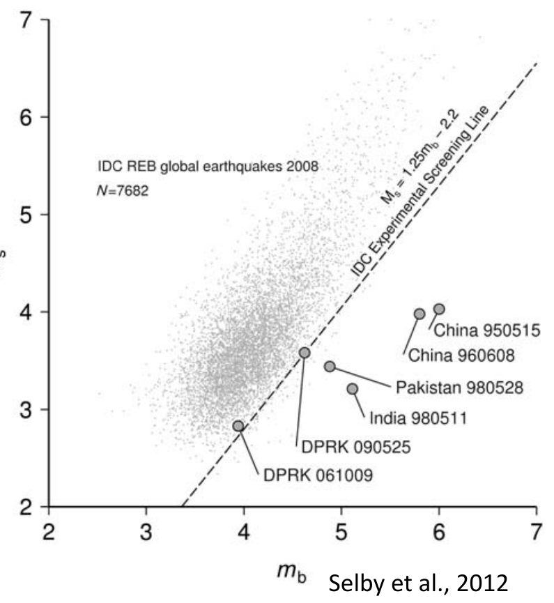
The world's earthquakes of 2008 (grey) and six explosions, with the screening line (dashed). North Korea's first two tests, 2006 and 2009, sit right on the line. These magnitudes come from the treaty organisation's own network, so they differ from this table's by a few tenths. Figure: Selby et al. (2012), shown in G. Ekström's "Seismology in MTV" slides (Columbia University, 2019).
The map below uses the same frame as that plot, mb and Ms from 2 to 7 at the same scale, with the screening line drawn on it, so the two can be laid side by side. It shows where the five fall against the model's probability everywhere. One seismic measure is never enough: agencies use several together, and a flag starts an investigation rather than ending one.
# the model's probability at every point of grid, the table of mb-Ms points made in the setup cell
grid_probability = model.predict_proba(grid[["mb", "Ms"]])[:, 1]

plt.figure(figsize=(7, 5.5))
plt.scatter(grid["mb"], grid["Ms"], c=grid_probability, cmap="coolwarm", s=12, marker="s")
plt.colorbar(label="probability of an explosion")
plt.scatter(korea["mb"], korea["Ms"], s=150, marker="*", color="yellow", edgecolor="black", label="North Korea")
plt.plot(mb_ends, mb_ends - gap, color="black", ls="--", label="line by eye")
plt.plot(mb_ends, 1.25 * mb_ends - 2.2, color="black", ls=":", label="treaty screening line, Ms = 1.25 mb - 2.2")
plt.xlim(2, 7)
plt.ylim(2, 7)
plt.gca().set_aspect("equal")     # the frame of the screening plot above
plt.xlabel("body-wave magnitude mb")
plt.ylabel("surface-wave magnitude Ms")
plt.title("The model's probability everywhere, with North Korea's explosions")
plt.legend(loc="upper left")
plt.show()
The question, answered
Mostly, with two magnitudes and an honest score. "Always earthquake" is right 0.895 of the time and finds nothing, so the scores count hits, misses and false alarms apart. A depth of 0 looks perfect only because the analyst already knew. A grid of 560 lines and logistic regression find nearly the same line through mb and Ms; the probability logistic regression adds lets the alarm be set on validation events, and on the test events, opened once, the rule catches 22 of 23 explosions with 0 false alarms. But at North Korea's small explosions the steep line misses what the plainer line catches: its slope was learned from large explosions.
Week 9 summary
The science
Earthquake or nuclear explosion?
When one label is rare, accuracy hides the misses: 'always earthquake' scores 0.895 and finds no explosion; precision, recall and F1 count the two kinds of mistake apart. Logistic regression draws a straight line through two columns and gives every event a probability; checked on events it never saw, the line through mb and Ms finds explosions that each magnitude alone misses. But its slope was learned from large explosions: at North Korea's small ones the plain line by eye does better. Where to set the alarm is a choice between missed explosions and false accusations; the ROC curve shows every choice at once, and a column that already knows the answer (a depth the analyst set to 0) is leakage, not skill.
- Body-wave and surface-wave magnitude. Two sizes for one event: mb is read from the first, fast P wave, Ms from the slow surface waves that follow. An explosion pushes out from one small spot and makes weak surface waves for its mb; an earthquake slips along a fault and makes strong ones.
- Baseline. Write the dumbest rule you can, first. Any model that cannot beat it is decoration.
- Hit, miss, false alarm. A hit is an explosion you flagged, a miss an explosion you did not, a false alarm an earthquake you flagged.
- Precision / recall. Of the ones you flagged, how many were right? Of the real ones, how many did you catch?
- Leakage. You got 99 percent. Be suspicious. Did one of your columns already know the answer?
- Logistic regression. The same straight line — but now it outputs a probability between 0 and 1.
- Decision boundary. Where the model's answer flips from one label to the other — for logistic regression, always a straight line.
- Alarm level. The probability at or above which you flag an event. Lower it and you miss fewer explosions but accuse more earthquakes.
- ROC curve. Every alarm level at once: the share of explosions caught against the share of earthquakes falsely flagged. The closer the curve hugs the top left, the better the model.
The code
| Function | What it does |
|---|---|
| Python | |
list.append(x) |
add one item to the end of a list |
len(table) |
how many rows |
for x in things: |
do the same thing once for each item |
round(x, 1) |
trim a long decimal — 9.1 rather than sixteen digits |
| NumPy | |
mask & other_mask |
True only where both masks are True, the array version of and |
np.array(list) |
the container that does arithmetic to every number at once |
| pandas | |
mask.mean() |
the proportion of a mask that is True, in one line |
| Matplotlib | |
plt.plot(x, y) |
join points with a line — here, the coastline |
plt.scatter(x, y) |
a dot per pair of values |
plt.hist(x, bins=n) |
how one list of numbers is spread out |
plt.axvline(x) |
a vertical line at x, to mark a boundary on a plot |
| scikit-learn | |
LogisticRegression() |
draw the straight line that best separates two labelled groups |
accuracy_score(y, pred) |
the fraction it got right — useless when one label is rare |
precision_score(y, pred) |
of the ones it flagged, how many really were explosions |
recall_score(y, pred) |
of the explosions there were, how many it flagged |
f1_score(y, pred) |
precision and recall in one number, so two models can be compared |
train_test_split(table, test_size=0.3, random_state=n, stratify=column) |
cut the rows into a training part and a held-out part, keeping the share of each label |
model.fit(X, y) / model.predict(X) |
learn from the training rows, then predict for any rows |
confusion_matrix(y, pred) |
the two kinds of mistake counted apart: misses in one corner, false alarms in the other |
model.predict_proba(X)[:, 1] |
the model's probability that each row is the True label |
roc_auc_score(y, prob) |
one number for the whole ROC curve: 1 is perfect, 0.5 is guessing |
Homework
An agency learns from the tests it knows and must watch places it has never recorded. Here you do the whole path of class again, alone: fit on the western US (405 events, 36 explosions, almost all at the Nevada Test Site), choose the alarm level on western-US validation events, and test once on Eurasia (Central Asia and Novaya Zemlya: 713 events, 81 explosions). One step of class per Your turn: the grid, the fit and the level, the test against the baselines, and the curve of every level. Each answer cell gives the names and says what each holds; you write the code.
The two tables come from events, which the setup cell makes: run the setup cell, then the next.
west_us = events[events["region"] == "western US"]
eurasia = events[events["region"] != "western US"]
eurasia_label = eurasia["is_explosion"]
slopes = np.arange(0.75, 2.5, 0.25).round(2)    # the grid of class
offsets = np.arange(0.05, 8.0, 0.1).round(2)
levels = [0.9, 0.7, 0.5, 0.3, 0.2, 0.1, 0.05]                          # the alarm levels of class
print(len(west_us), "events in the western US;", len(eurasia), "in Eurasia")
✏️ Your turn 12
Which line does a grid find on the western training events?
Why: the search of Your turn 6, alone, on new events.
west_train,west_validation: the western-US events cut 70/30, stratified on their label,random_state=42.west_f1s: for every offset inoffsetsand every slope inslopes(class's grid, set again at the top of the homework), the training F1 of the line Ms < slope × mb − offset.west_best_f1,west_best_slope,west_best_offset: kept inside the loop, as in Your turn 6. The last line, given, counts how many lines share the best F1.
Use these names, because the self-check looks for them: west_train, west_best_slope and
west_best_offset.
# ← your answer here: replace every ... with code
west_train, west_validation = ...  # the western-US events, 30 percent to validation, stratified, random_state=42
west_f1s = []
west_best_f1 = 0
for offset in offsets:
    for slope in slopes:
        f1_west = ...              # this line's F1 on the western training events
        ...                        # append it to west_f1s
        ...                        # if it beats west_best_f1, keep its F1, slope and offset
print("the western grid's line: Ms <", west_best_slope, "x mb -", west_best_offset, ", training F1", round(west_best_f1, 3))
print(west_f1s.count(west_best_f1), "lines share that F1")
# Self-check: run this after your answer. You do not need to read it — it only says whether something is off.
assert len(west_train) == 283 and west_train["is_explosion"].sum() == 25, "west_us cut 70/30, stratified on its label, random_state=42"
assert (west_best_slope, west_best_offset) == (1.75, 5.05), "the pair at the position of the largest F1 in west_f1s"
print(f"✓ Your turn 12 — the western grid's line: Ms < {west_best_slope} x mb - {west_best_offset}")
What the numbers mean. Several lines share the best F1. Why does that happen here and not in class, and what does it say about choosing a line from so few explosions?
✏️ Your turn 13
Fitted in the west, which alarm level does the western validation choose?
Why: the steps of Your turns 7 and 9, alone: fit on training events, choose on validation events, before the test region is looked at.
model_west: logistic regression fitted onwest_train's mb and Ms and label.west_level_f1s: for each level inlevels(class's levels), the F1 onwest_validationof flagging the events whose probability is at or above it.west_level: the level with the best F1.
Use these names, because the self-check looks for them: model_west, west_level_f1s and
west_level.
# ← your answer here: replace every ... with code
model_west = ...     # logistic regression fitted on the western training events
prob_west_val = ...  # its probability for each western validation event
west_level_f1s = []
for level in levels:
    ...              # append the western validation F1 at this level
    print("level", level, ": western validation F1", round(west_level_f1s[-1], 3))
west_level = ...     # the level with the best F1 in your printout
# Self-check: run this after your answer. You do not need to read it — it only says whether something is off.
assert [round(x, 3) for x in west_level_f1s] == [0.0, 0.429, 0.706, 0.9, 0.909, 0.667, 0.468], "F1 on west_validation of prob >= level, the model fitted on west_train"
assert west_level == 0.2, "the level with the largest F1"
print(f"✓ Your turn 13 — the level chosen on western validation: {west_level}")
What the numbers mean. How many explosions decide this choice? How sure can you be of it?
✏️ Your turn 14
Opened once: how do the western rules do in Eurasia?
Why: Eurasia is the test region. Every choice is made; this is the number to report.
prob_eurasia:model_west's probability for every Eurasian event.eurasia_countsandeurasia_f1: the confusion matrix and the F1 of flagging atwest_level.eurasia_f1_grid: the F1 in Eurasia of the western grid's line.eurasia_accuracyandeurasia_f1_mb: the baselines of Your turns 1 and 2 in Eurasia: the accuracy of "always earthquake", by hand, and the F1 of the cut at mb 5.7.
Use these names, because the self-check looks for them: eurasia_counts, eurasia_f1,
eurasia_f1_grid, eurasia_accuracy and eurasia_f1_mb.
# ← your answer here: replace every ... with code
prob_eurasia = ...      # the western model's probability for each Eurasian event
eurasia_counts = ...    # the confusion matrix in Eurasia at west_level
eurasia_f1 = ...        # the F1 in Eurasia at west_level
eurasia_f1_grid = ...   # the F1 in Eurasia of the western grid's line
eurasia_accuracy = ...  # the share of Eurasian events that are earthquakes
eurasia_f1_mb = ...     # the F1 in Eurasia of the cut at mb 5.7
print(eurasia_counts)
print("Eurasia F1: logistic regression at", west_level, ":", round(eurasia_f1, 3), "  the western grid's line:", round(eurasia_f1_grid, 3))
print("baselines: always earthquake, accuracy", round(eurasia_accuracy, 3), "  the cut on mb, F1", round(eurasia_f1_mb, 3))
# Self-check: run this after your answer. You do not need to read it — it only says whether something is off.
assert eurasia_counts[1, 1] == 77 and eurasia_counts[0, 1] == 12, "flag Eurasia where prob_eurasia >= west_level"
assert round(eurasia_f1, 3) == 0.906, "f1_score of eurasia_label and those flags"
assert round(eurasia_f1_grid, 3) == 0.938, "Ms < west_best_slope * mb - west_best_offset, in Eurasia"
assert round(eurasia_accuracy, 3) == 0.886 and round(eurasia_f1_mb, 3) == 0.667, "the share of earthquakes; the F1 of eurasia['mb'] >= 5.7"
print(f"✓ Your turn 14 — Eurasia F1: {eurasia_f1:.3f} for logistic regression, {eurasia_f1_grid:.3f} for the grid's line")
What the numbers mean. The level was chosen on western events. Did it suit Eurasia? Why might a level chosen at one site not suit another?
✏️ Your turn 15
How good is the western model in Eurasia at every alarm level at once?
Why: the ROC curve of class, in the new place, and its area computed by hand: the area is the share of (explosion, earthquake) pairs that the model puts in the right order, explosion higher.
eurasia_hit_sharesandeurasia_false_alarm_shares: for each level inroc_levels, the share of Eurasia's explosions flagged and the share of its earthquakes flagged.auc_by_hand: over every explosion, count the earthquakes with a lower probability; add the counts; divide by (number of explosions × number of earthquakes). The next line printsroc_auc_scorebeside it.- The figure: the curve and the diagonal.
Use these names, because the self-check looks for them: eurasia_hit_shares,
eurasia_false_alarm_shares and auc_by_hand.
# ← your answer here: replace every ... with code
roc_levels = [1.0, 0.9, 0.7, 0.5, 0.3, 0.2, 0.1, 0.05, 0.02, 0.01, 0.0]  # more levels than class, for a smoother curve
eurasia_hit_shares = []
eurasia_false_alarm_shares = []
for level in roc_levels:
    flagged = ...                                                        # Eurasian events at or above this level
    eurasia_hit_shares.append(...)                                       # the share of Eurasia's explosions flagged
    eurasia_false_alarm_shares.append(...)                               # the share of Eurasia's earthquakes flagged

prob_explosions = ...   # the probabilities of Eurasia's explosions
prob_earthquakes = ...  # the probabilities of Eurasia's earthquakes
pairs_right = 0
for p in prob_explosions:
    pairs_right = ...   # add the number of earthquakes with a probability below p
auc_by_hand = ...       # the share of (explosion, earthquake) pairs in the right order
print("area under the curve: by hand", round(auc_by_hand, 3), "  roc_auc_score", round(roc_auc_score(eurasia_label, prob_eurasia), 3))

plt.figure(figsize=(5.5, 5.5))
plt.plot(eurasia_false_alarm_shares, eurasia_hit_shares, marker="o", color="black", label="model fitted in the western US")
plt.plot([0, 1], [0, 1], color="0.6", ls="--", label="a coin toss")
plt.xlabel("share of earthquakes falsely flagged")
plt.ylabel("share of explosions caught")
plt.title("ROC curve in Eurasia")
plt.legend()
plt.show()
# Self-check: run this after your answer. You do not need to read it — it only says whether something is off.
assert [round(x, 3) for x in eurasia_hit_shares] == [0.0, 0.123, 0.58, 0.84, 0.938, 0.951, 0.988, 0.988, 1.0, 1.0, 1.0], "for each level: flagged explosions over Eurasia's explosions"
assert [round(x, 3) for x in eurasia_false_alarm_shares] == [0.0, 0.0, 0.0, 0.0, 0.006, 0.019, 0.092, 0.318, 0.672, 0.856, 1.0], "flagged earthquakes over Eurasia's earthquakes"
assert round(auc_by_hand, 3) == 0.992, "pairs in the right order over explosions times earthquakes"
print(f"✓ Your turn 15 — area under the ROC curve in Eurasia: {auc_by_hand:.3f}")
What the numbers mean. The area is close to 1, yet the line still missed explosions at the level chosen in the west. How can both be true?