Where was this basalt made?
EPS 88 · PyEarth. Open your own copy on DataHub: click here.
Basalt is the commonest volcanic rock on Earth: the crust under every ocean is made of it. It is made in three different places, where the mantle melts, and a geologist often holds a piece without knowing which. California's Coast Ranges, for example, hold slices of old sea floor lifted onto the continent, and whether that crust was made at a mid-ocean ridge or above a sinking plate decides what story the rocks tell. The rock cannot say where it came from. Its chemistry can.
Today you work with 756 basalts whose birthplace is known, compiled by the geologist Pieter Vermeesch (2006) from published analyses. You start with last week's logistic regression, then ask the week's real question: will a model work on rocks it has never seen? Cross-validation answers it, and with it you judge two new models, a random forest and a support vector machine. Nearly a third of the rocks are locked away at the start and opened once, at the end. At home you ask whether the winner works on rocks from somewhere else.
Every place you write something opens with a pencil icon and the words Your turn, and is
followed by a cell that already has the shape of the answer written in, with ... wherever your
code goes. Replace every ..., run every cell so your answers and figures are
saved in the file, then download this notebook itself — the .ipynb file — and upload it
to Gradescope. Not a PDF: the marking reads your notebook, and a PDF cannot be read.
In JupyterLab: File ▸ Download, or right-click the file in the left-hand panel and choose
Download.
Two habits from the first minute. A cell runs when you press Shift+Enter, and the notebook remembers everything it has already run — so when something breaks and you cannot see why, Kernel → Restart Kernel and Run All Cells throws the memory away and rebuilds it from the top. That is never the wrong thing to do.
What you'll be able to do
The science. Name the three places basalt melts and why, and say which element tells them apart best.
The code. Last week's LogisticRegression and confusion_matrix, now with three settings ·
training, validation and test, each with one job · cross-validation with cross_val_score ·
DecisionTreeClassifier and RandomForestClassifier · SVC, with StandardScaler and
make_pipeline · the best tree depth picked with np.argmax · every model scored once on the sealed
rocks.
The five questions of the class, then the three classifiers compared:
- What in a basalt's chemistry records where it was made?
- How well does last week's model sort the rocks?
- Which model will work best on rocks it has not seen?
- Can a random forest beat last week's lines?
- Can a support vector machine beat them?
Setup
Run the next cell once. It reads the basalts, stored with the course: one row per rock, its
setting (where it was made; section 1 explains) and its chemistry. Two columns are renamed so every
name follows one pattern (the file calls the setting affinity), and one
impossible value is blanked (a rock recorded with 19 percent MnO; basalt holds well under 1
percent).
import numpy as np
from sklearn.linear_model import LogisticRegression
from sklearn.ensemble import RandomForestClassifier
from sklearn.svm import SVC
from sklearn.preprocessing import StandardScaler
from sklearn.pipeline import make_pipeline
from sklearn.tree import DecisionTreeClassifier, export_text
from sklearn.model_selection import train_test_split, cross_val_score
from sklearn.metrics import confusion_matrix, ConfusionMatrixDisplay
import pandas as pd
import matplotlib.pyplot as plt

# house style, set once, so every plot cell below holds only what matters
plt.rcParams.update({"figure.dpi": 110,
                     "axes.grid": True, "grid.alpha": 0.3, "axes.axisbelow": True})

CACHE = "https://raw.githubusercontent.com/AI4EPS/EPS88_PyEarth/main/data"

# One row per rock: its setting (IAB, MORB or OIB) and up to 51 chemical measurements.
# Source: Vermeesch (2006), Geochemistry, Geophysics, Geosystems 7, doi:10.1029/2005GC001092.
rocks = pd.read_csv(CACHE + "/week10_vermeesch_basalts.csv")
rocks = rocks.rename(columns={"affinity": "setting", "P2O5(wt%)": "P2O5_wt_percent"})
rocks.loc[rocks["MnO_wt_percent"] > 5, "MnO_wt_percent"] = np.nan   # one impossible value, blanked
print(len(rocks), "rocks,", rocks.shape[1] - 1, "measurements each (many blank)")
1. What in a basalt's chemistry records where it was made?
A rock with no address. California's Coast Ranges hold slices of old sea floor, scraped off a sinking plate and lifted onto the continent. Was that crust made at a mid-ocean ridge, above a sinking plate, or on an ocean island? The answer decides the history the rocks tell, and the rock itself cannot say. Its chemistry can.
Basalt has three main homes in the ocean. Basalt is made in three places, where the mantle melts: where two plates pull apart (a mid-ocean ridge), where one plate sinks under another (an island arc), and over a hot plume, usually far from any plate edge (an ocean island). (It also forms on
the continents, where they rift apart or flood with lava; today's rocks come from the three ocean homes.)
Geologists call the kind of place a rock was made its tectonic setting. In the data it is the
column setting, with three values named after the rock: IAB (island-arc basalt), MORB
(mid-ocean-ridge basalt) and OIB (ocean-island basalt).
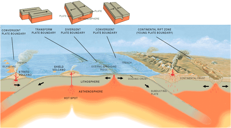
Among its features: an island arc above a sinking plate, a shield volcano over a hot spot, and a mid-ocean ridge where two plates pull apart. Cross-section by José F. Vigil, USGS (public domain), via Wikimedia Commons.
From the outside the three look alike: dark fine-grained rock, often in rounded "pillows" where lava met cold sea water:
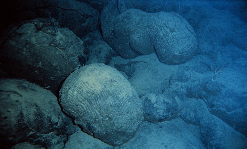
Pillow basalt on the sea floor. Photo: NOAA (public domain), via Wikimedia Commons.
So geologists measure what is inside. A rock analysis gives the common elements as oxides, in percent of the rock's weight (SiO2, TiO2), and the rare ones in parts per million (V, Sr).
First, lock some rocks away. The routine analysis of a rock lists nine major oxides: silica, titanium, aluminium, calcium, magnesium, manganese, potassium, sodium and phosphorus. (Iron is left out: more than half of all 756 rocks have no iron value, and the rest split it between FeO and Fe2O3 in different ways.) The next cell keeps the 640 rocks with all nine and, as in the model-selection week, splits them once: 448 training rocks to build and choose with, and 192 sealed rocks that nothing touches until the last Your turn of class. A score on rocks that helped choose the model is not a test, so from here on even our first look at the data uses the training rocks only.
oxides = ["SiO2_wt_percent", "TiO2_wt_percent", "Al2O3_wt_percent", "CaO_wt_percent", "MgO_wt_percent",
          "MnO_wt_percent", "K2O_wt_percent", "Na2O_wt_percent", "P2O5_wt_percent"]
rocks_ox = rocks.dropna(subset=oxides)   # rocks with all nine oxides measured
train, sealed = train_test_split(rocks_ox, test_size=0.3, random_state=0, stratify=rocks_ox["setting"])
print(len(train), "training rocks,", len(sealed), "sealed until the end")
What is basalt made of? The next cell takes the middle (median) training rock, oxide by oxide, and draws it.
middle = train[oxides].median().sort_values()   # the median of each oxide, smallest first
plt.figure(figsize=(7, 3.5))
plt.barh(middle.index, middle)
plt.xlabel("weight percent of the rock")
plt.title("The middle training basalt")
plt.show()
print("the nine add up to", round(middle.sum()), "percent")
Half of basalt is silica. The middle rock holds 49.6 percent SiO2, then 15.6 Al2O3, 11.0 CaO, 7.5 MgO and 2.6 Na2O; most of the missing 11 percent is the iron left out above. These big five are what basalt's minerals are built from: olivine and pyroxene (magnesium, iron, silica; pyroxene also much of the calcium) and feldspar (aluminium, calcium, sodium, silica). The other four are small: 1.4 percent TiO2, 0.5 K2O, and P2O5 and MnO about 0.2 each.
Think before you run the next cell. The three homes melt the same kind of mantle, in different ways. Which oxides would you expect to differ between the homes: the big ones that build the minerals, or the small ones? The cell prints each oxide's median in each setting, then, for each oxide, the largest of the three medians divided by the smallest.
by_setting = train.groupby("setting")[oxides].median()   # one row per setting, one column per oxide
print(by_setting.T.round(2))                              # .T turns it: one row per oxide
spread = np.max(by_setting, axis=0) / np.min(by_setting, axis=0)   # largest median over smallest, down each column
print(spread.sort_values().round(1))
The big oxides barely move; three small ones do. Silica's median runs only from 46.8 to 50.1 percent across the three settings, and no big oxide's largest median is even one and a half times its smallest. Phosphorus differs 2.9 times, titanium 3.1 times, potassium 5.9 times. Why these three?
Each home melts the mantle in its own way, and the melt keeps the mark. Titanium, potassium and phosphorus fit badly into the mantle's minerals, so they prefer the melt. When only a little of the mantle melts, what there is of them gathers into a little liquid and the basalt is rich in them; when much melts, they are diluted. The table follows titanium and potassium, the two that differ most.
| Home | Why the mantle melts | How much melts | Titanium | Potassium | Examples |
|---|---|---|---|---|---|
| Mid-ocean ridge (MORB) | the plates pull apart; hot mantle rises to fill the gap and melts as the pressure on it drops | a large share | middle: diluted in much melt | low: this mantle lost it in melts long ago | Mid-Atlantic Ridge, East Pacific Rise |
| Island arc (IAB) | water from the sinking plate lowers the mantle's melting point, as salt melts ice | varies | low: this mantle has often melted before, and the water brings little | raised: the water carries it, with strontium, out of the sinking plate; some arcs (Tonga, Izu-Bonin) still hold little | Mariana, Izu-Bonin, Tonga, Aleutians |
| Ocean island (OIB) | a plume of unusually hot mantle rises, usually far from any plate edge; the thick plate above stops it rising far | a small share, deep down, of a mantle richer in both elements | high | highest | Hawaii, Samoa, the Canary Islands |
Read the table against the medians you printed. The middle arc rock holds 0.9 percent TiO2 and 0.51 percent K2O; the middle ridge rock 1.42 and 0.16; the middle ocean-island rock 2.78 and 0.94. Titanium puts all three in order; potassium helps where titanium overlaps, ridge from arc at low titanium and ridge from ocean island at high. Phosphorus behaves like potassium without the arc's water (0.14, 0.14 and 0.4): raised only in the islands.
Geologists have drawn lines between the settings by hand since the 1980s, on plots of two elements such as these; the homework meets the most famous one.
The bar. Write the dumbest rule you can, first. Any model that cannot beat it is decoration. The next cell counts the training rocks in each setting
(value_counts lists the commonest first) and scores the guess "always the commonest setting".
counts = train["setting"].value_counts()
print(counts)
print("guess the commonest setting every time: right", round(counts.iloc[0] / len(train), 3), "of the time")
0.355, the score to beat. Last week, when explosions were rare, the share right hid the misses, and you counted them apart. Here the three settings are nearly equal in number (159, 151 and 138 training rocks), so the share right is a fair score; the confusion matrix still shows where the misses fall. The next cell draws the training rocks on the two elements the first models use.
ti_k = ["TiO2_wt_percent", "K2O_wt_percent"]   # the names of the titanium and potassium columns
plt.figure(figsize=(7, 4.5))
for setting, marker in [("IAB", "o"), ("MORB", "s"), ("OIB", "^")]:
    some = train[train["setting"] == setting]
    plt.scatter(some["TiO2_wt_percent"], some["K2O_wt_percent"], s=12, marker=marker, label=setting)
plt.xlabel("TiO2 (weight percent)")
plt.ylabel("K2O (weight percent)")
plt.title("The training rocks")
plt.legend()
plt.show()
2. How well does last week's model sort the rocks?
Last week's logistic regression, in last week's symbols. For each event it worked out one number, $z$, from the two magnitudes, and bent $z$ into a probability with the S-curve:
$$p = \frac{1}{1 + e^{-z}}, \qquad z = a \times \text{mb} + b \times \text{Ms} + c$$
$p$ is the probability that the event is an explosion, and fit chose the three numbers $a$, $b$
and $c$. Where $z = 0$, $p = 0.5$: those events lie on a straight line, the decision boundary, with
explosions predicted on one side and earthquakes on the other.
With three settings, three z's. For a rock with titanium Ti and potassium K (both in weight percent), the model works out one $z$ for each setting:
$$z_{\text{IAB}} = a_1 \times \text{Ti} + b_1 \times \text{K} + c_1, \quad z_{\text{MORB}} = a_2 \times \text{Ti} + b_2 \times \text{K} + c_2, \quad z_{\text{OIB}} = a_3 \times \text{Ti} + b_3 \times \text{K} + c_3$$
It turns the three into three probabilities that add up to 1, and predicts the setting with the
largest. Where two settings' $z$'s are equal, a straight line runs between them, so the map is cut
into three regions with straight edges. fit now chooses nine numbers instead of three.
✏️ Your turn 1
How well does last week's model sort the training rocks on titanium and potassium?
Why: last week's model, scored last week's way, is where every new model starts.
line_tk: aLogisticRegression(max_iter=5000)fitted on the training rocks' titanium and potassium,train[ti_k](ti_kholds the two column names, from the scatter cell above), and their setting,train["setting"]. We call it "the lines", for the straight edges it draws.counts_tk: its confusion matrix, as last week: the true settings, then the model's predictions for the same rocks. Three settings make three rows (the truth) and three columns (the prediction); the given lines draw it.score_tk: the share predicted right, from the diagonal ofcounts_tkandlen(train). The library's.score(given) does the same count; from here on we use it.
Use these names, because the self-check looks for them: line_tk, counts_tk and score_tk.
# ← your answer here: replace every ... with code
# train: the 448 training rocks; ti_k: the names of the TiO2 and K2O columns
line_tk = LogisticRegression(max_iter=5000)                            # max_iter: more fitting steps than the default 100
line_tk.fit(..., ...)                                                  # the training rocks' TiO2 and K2O, and their setting
counts_tk = confusion_matrix(..., ..., labels=["IAB", "MORB", "OIB"])  # true settings, then the model's predictions
plt.figure(figsize=(4.5, 4))
ConfusionMatrixDisplay(counts_tk, display_labels=["IAB", "MORB", "OIB"]).plot(ax=plt.gca(), cmap="Blues", colorbar=False)
plt.grid(False)
plt.title("The lines on Ti and K, training rocks")
plt.show()
score_tk = ...                                                         # the diagonal, counts_tk[0, 0] + counts_tk[1, 1] + counts_tk[2, 2], over the number of training rocks
library_score = line_tk.score(train[ti_k], train["setting"])
print("the lines on titanium and potassium:", round(score_tk, 3), "of the training rocks right")
print("the library's .score says:", round(library_score, 3))
# Self-check: run this after your answer. You do not need to read it — it only says whether something is off.
assert (np.array(counts_tk) == np.array([[135, 18, 6], [15, 128, 8], [1, 14, 123]])).all(), "the true settings first, then line_tk's predictions for the same training rocks"
assert round(score_tk, 3) == 0.862, "the three counts on the diagonal, added, over the number of training rocks"
print(f"✓ Your turn 1 — the lines get {score_tk:.3f} of the training rocks right")
0.862, against 0.355 for a guess. Read the matrix row by row, as last week's recall: of 159 arc rocks it predicts 135 right, of 151 ridge rocks 128, of 138 ocean-island rocks 123. Of its 62 misses, 33 are arcs and ridges mistaken for each other. Last week each event got one probability, of being an explosion; now each rock gets three, one per setting, adding up to 1:
one_rock = train.loc[[59], ti_k]   # one training rock, picked by its index label
print(one_rock)
probabilities = line_tk.predict_proba(one_rock)[0]   # one probability per setting
print("probabilities", line_tk.classes_, ":", probabilities.round(2))
print("they add up to", probabilities.sum().round(2))
print("predicted:", line_tk.predict(one_rock)[0])
0.27, 0.71 and 0.01: the model predicts the largest,
MORB (the rock is MORB). What regions did the model draw? The next cell
writes a small function, draw_regions, that asks a fitted model to predict the setting at every
point of a fine grid of titanium and potassium values, and colours the map by its predictions; the
lines around it open and show the figure. It is used again in sections 4 and 5, for the new models.
def draw_regions(model, title):
    """Colour a TiO2-K2O map by what a fitted model predicts at each point, and draw the training rocks on it."""
    # 1. a grid of made-up rocks, every 0.05 percent of TiO2 and of K2O
    ti_grid, k_grid = [], []
    for ti in np.arange(0, 4.51, 0.05):
        for k in np.arange(0, 3.01, 0.05):
            ti_grid.append(ti)
            k_grid.append(k)
    grid = pd.DataFrame({"TiO2_wt_percent": ti_grid, "K2O_wt_percent": k_grid})
    # 2. the model's prediction for each made-up rock
    predicted = model.predict(grid)
    # 3. colour each made-up rock by its prediction, and draw the real training rocks on top
    for setting, colour, light in [("IAB", "tab:blue", "#c6dbef"), ("MORB", "tab:orange", "#fdd0a2"), ("OIB", "tab:green", "#c7e9c0")]:
        here = predicted == setting             # the made-up rocks predicted as this setting
        plt.scatter(grid["TiO2_wt_percent"][here], grid["K2O_wt_percent"][here], s=30, marker="s", color=light, lw=0)
        some = train[train["setting"] == setting]   # and the real training rocks of this setting
        plt.scatter(some["TiO2_wt_percent"], some["K2O_wt_percent"], s=12, color=colour, edgecolor="black", lw=0.3, label=setting)
    plt.xlabel("TiO2 (weight percent)")
    plt.ylabel("K2O (weight percent)")
    plt.title(title)
    plt.grid(False)                             # no grid lines over the coloured map
    plt.legend()

plt.figure(figsize=(7, 4.5))
draw_regions(line_tk, "The lines on Ti and K: three regions with straight edges")
plt.show()
Three regions with straight edges, each edge where two settings' $z$'s tie. Most rocks sit in the region of their own colour; the arc and ridge rocks at low titanium overlap, and no straight edge can part them.
More columns: all nine oxides. The next cell names the nine oxides of every training rock X
and their settings y, fits the same model on X, and scores it on the training rocks beside
the two-element model.
X = train[oxides]      # the nine oxides of every training rock
y = train["setting"]   # and its setting
line_nine = LogisticRegression(max_iter=5000)
line_nine.fit(X, y)
train_score_tk = line_tk.score(train[ti_k], y)
train_score_nine = line_nine.score(X, y)
print("the lines on Ti and K:     ", round(train_score_tk, 3), "of the training rocks right")
print("the lines on nine oxides:  ", round(train_score_nine, 3))
0.922 against 0.862. Are nine oxides better? These training scores cannot say. Both are scores on the rocks the models learned from. A model with more columns has more ways to fit those very rocks, accidents and all, so a training score flatters it. What we want is how a model does on rocks it has never seen: how well it generalizes. The next section measures that.
3. Which model will work best on rocks it has not seen?
Three sets of rocks, each with one job. You met these in the model-selection week:
| Set | Rocks here | Its one job |
|---|---|---|
| training | rocks the model learns from | fit the model |
| validation | training rocks held out from the fit | choose between models |
| test | the 192 sealed rocks | report the chosen model's score, once |
The sealed rocks cannot help choose: a score used to choose is no longer a test. So the choice is made on validation rocks taken out of the 448 training rocks.
Which fifth to hold out for validation? The next cell holds out a different random fifth of the training rocks 20 times. Each time it fits the nine-oxide lines on the other four fifths and scores them on the fifth held out.
split_scores = []
for seed in range(20):
    fit_80, held_20 = train_test_split(train, test_size=0.2, random_state=seed, stratify=train["setting"])
    model = LogisticRegression(max_iter=5000)
    model.fit(fit_80[oxides], fit_80["setting"])
    split_scores.append(model.score(held_20[oxides], held_20["setting"]))

plt.figure(figsize=(7, 3))
plt.scatter(range(20), split_scores)
plt.xticks(range(0, 20, 2))
plt.xlabel("random split number (random_state)")
plt.ylabel("share right on the held-out fifth")
plt.title("One model, 20 validation splits of the 448 training rocks")
plt.show()
print("lowest", round(np.min(split_scores), 3), " highest", round(np.max(split_scores), 3))
The same model scores anywhere from 0.867 to 0.967, depending only on which rocks were held out. With one validation split, a difference of a few points between two models can be nothing but the luck of the split.
Cross-validation fixes this. Cut the rows into five parts; hold out each part in turn, train on the other four, and score on the one held out. Five scores, and every row tested once.
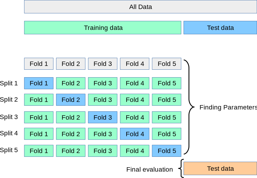
Top: all the rocks, split once into training rocks and the sealed test rocks. Middle: the training rocks cut into five parts (the figure calls them folds); in each of the five splits one part (blue) is held out and scored, and the model is fitted on the other four (green). The mean of the five scores is the model's cross-validation score, and it is what models are chosen by. Bottom: the chosen model is scored once on the test rocks. Figure: scikit-learn documentation (BSD licence).
The library does all five rounds in one line:
scores = cross_val_score(model, X, y, cv=5)
model is a new, unfitted model; X the columns and y the labels of the training rocks; cv=5
asks for five parts. The library cuts the parts itself, keeping each setting's share the same in
every part, then fits and scores five times and returns the five scores, one per round.
✏️ Your turn 2
What does the nine-oxide model score on rocks it did not learn from?
Why: a training score flatters a model; a cross-validation score is how it does on rocks held out. This is the score every model is judged by from here on.
nine_scores: the five cross-validation scores ofline_nine, the nine-oxide lines from the cell above, onXandy, with five parts. (cross_val_scorefits its own fresh copy of the model in each round; the model you hand it is left as it was.)nine_cvandnine_spread: the mean and the standard deviation of the five scores.
The last print sets the mean beside the training score from the cell above.
Use these names, because the self-check looks for them: nine_scores and nine_cv.
# ← your answer here: replace every ... with code
# X, y, line_nine, train_score_nine: the nine oxides, the setting, the lines and their training score, from above
nine_scores = cross_val_score(..., ..., ..., cv=5)  # the nine-oxide lines, then the nine oxides and the setting
nine_cv = np.mean(...)                              # the mean of the five scores
nine_spread = np.std(...)                           # their standard deviation
print("five held-out scores:", np.round(nine_scores, 3))
print("mean", round(nine_cv, 3), "  spread", round(nine_spread, 3))
print("training score", round(train_score_nine, 3), "  cross-validation mean", round(nine_cv, 3))
# Self-check: run this after your answer. You do not need to read it — it only says whether something is off.
assert [round(s, 3) for s in nine_scores] == [0.878, 0.911, 0.911, 0.921, 0.888], "cross_val_score(line_nine, X, y, cv=5)"
assert round(nine_cv, 3) == 0.902, "the mean of the five scores"
print(f"✓ Your turn 2 — the lines on nine oxides: {nine_cv:.3f} by cross-validation")
Five scores, from 0.878 to 0.921, mean 0.902: below the training score, 0.922. That gap is what the training score hid. The spread of the five, 0.016, says how much one part's luck can move a score. Now the question the training scores could not answer.
✏️ Your turn 3
Do nine oxides generalize better than titanium and potassium?
Why: this is what cross-validation is for: choosing between models by how they do on rocks they did not learn from.
tk_scores: the five cross-validation scores ofline_tk, your lines from Your turn 1, on the training rocks' titanium and potassium,train[ti_k], andy.tk_cv: their mean.nine_cvis yours from Your turn 2.
Use these names, because the self-check looks for them: tk_scores and tk_cv.
# ← your answer here: replace every ... with code
# line_tk: Your turn 1; nine_scores, nine_cv: the nine-oxide lines' five scores and their mean, from Your turn 2
tk_scores = cross_val_score(..., ..., ..., cv=5)  # line_tk, then the training rocks' TiO2 and K2O, and their setting
tk_cv = np.mean(...)                              # the mean of the five scores
print("Ti and K:   ", np.round(tk_scores, 3), " mean", round(tk_cv, 3))
print("nine oxides:", np.round(nine_scores, 3), " mean", round(nine_cv, 3))
# Self-check: run this after your answer. You do not need to read it — it only says whether something is off.
assert round(tk_cv, 3) == 0.868, "the lines on train[ti_k] and y, cv=5, then the mean"
print(f"✓ Your turn 3 — Ti and K {tk_cv:.3f}, nine oxides {nine_cv:.3f}")
Yes: 0.902 against 0.868, and the nine oxides win on 4 of the 5 parts. Held out, titanium and potassium score about what they scored on the training rocks (0.862): two columns leave little room to fit accidents. The nine oxides lose 2.0 points of their training score but keep the lead. 0.902, the lines on nine oxides, is now the bar every new model must beat.
4. Can a random forest beat last week's lines?
A random forest is a vote of many decision trees. So first, one tree.
One tree. A flowchart of yes/no questions, learned from the data instead of written by hand. It works like a geologist's flowchart. The next cell grows a tree only two questions deep on titanium and potassium and prints it. Each question is the one that leaves the rocks on its two sides least mixed.
tree_2 = DecisionTreeClassifier(max_depth=2, random_state=0)   # at most two questions deep
tree_2.fit(train[ti_k], y)
print(export_text(tree_2, feature_names=ti_k))
tree_2_train = tree_2.score(train[ti_k], y)
tree_2_scores = cross_val_score(DecisionTreeClassifier(max_depth=2, random_state=0), train[ti_k], y, cv=5)
tree_2_cv = np.mean(tree_2_scores)
print("on the training rocks:", round(tree_2_train, 3), "  cross-validation mean:", round(tree_2_cv, 3))
Read it from the top, as a flowchart. Is TiO2 at most 2.13 percent? If yes: is it at most 1.04? Then arc, else ridge. If no: is K2O at most 0.17 percent? Then ridge, else ocean island. Follow a rock with 1.07 percent TiO2 and 0.1 percent K2O: the tree predicts MORB (it is MORB). Titanium first, as in the melting table, and potassium to part ridge from island at high titanium. This little tree gets 0.801 of the training rocks right and 0.779 by cross-validation, below the lines' 0.868.
A deeper tree asks more questions and can follow the rocks more closely. How deep should it go?
✏️ Your turn 4
How deep should a tree be?
Why: a deeper tree always fits its training rocks better. Cross-validation says whether it also does better on rocks held out, and so chooses the depth.
tree_train_scoresandtree_cv_meansstart as empty lists (given).- For each
depthindepths(1 to 12):tree: aDecisionTreeClassifier(max_depth=depth, random_state=0)fitted ontrain[ti_k]andy; append its score on those same rocks totree_train_scores;tree_scores: the five cross-validation scores of a new tree of the same depth ontrain[ti_k]andy; append their mean totree_cv_means.
- Plot both lists against
depths, with a legend. best_depth: the depth with the highest cross-validation mean.np.argmax(values)gives the position of the largest value, as in the model-selection week.
Use these names, because the self-check looks for them: tree_train_scores, tree_cv_means
and best_depth.
# ← your answer here: replace every ... with code
depths = range(1, 13)
tree_train_scores = []
tree_cv_means = []
for depth in ...:                  # each depth from 1 to 12
    tree = DecisionTreeClassifier(max_depth=..., random_state=0)
    tree.fit(..., ...)             # the training rocks' TiO2 and K2O, and their setting
    tree_train_scores.append(...)  # its score on those same rocks
    tree_scores = cross_val_score(DecisionTreeClassifier(max_depth=..., random_state=0), ..., ..., cv=5)  # a new tree of this depth, five parts
    tree_cv_means.append(...)      # the mean of the five scores

plt.figure(figsize=(7, 4))
plt.plot(..., ..., marker="o", label="training score")         # depth, then the training scores
plt.plot(..., ..., marker="s", label="cross-validation mean")  # depth, then the cross-validation means
plt.xlabel("max_depth (questions deep)")
plt.ylabel("share of rocks right")
plt.title("One tree on Ti and K, 448 training rocks")
plt.legend()
plt.show()
best_depth = depths[np.argmax(...)]                            # the position of the highest cross-validation mean
print("best depth by cross-validation:", best_depth, "  its mean:", round(np.max(tree_cv_means), 3))
# Self-check: run this after your answer. You do not need to read it — it only says whether something is off.
assert len(tree_train_scores) == 12 and len(tree_cv_means) == 12, "one score of each kind per depth, 1 to 12"
assert [round(s, 3) for s in tree_train_scores] == [0.609, 0.801, 0.806, 0.891, 0.906, 0.929, 0.953, 0.967, 0.982, 0.991, 0.998, 1.0], "each tree scored on the same training rocks it was fitted on"
assert [round(s, 3) for s in tree_cv_means] == [0.612, 0.779, 0.772, 0.806, 0.833, 0.824, 0.817, 0.803, 0.806, 0.817, 0.81, 0.812], "the mean of cross_val_score for a new tree of each depth, cv=5"
assert best_depth == 5, "the depth at the position of the highest cross-validation mean"
print(f"✓ Your turn 4 — best depth {best_depth}, cross-validation mean {np.max(tree_cv_means):.3f}")
The training score climbs from 0.609 to 1.000; the cross-validation mean peaks at 0.833 at depth 5, then falls to about 0.812. Past depth 5 the tree learns the training rocks themselves, odd ones included, rather than the pattern behind them. That is overfitting: the training score cannot see it, because it only gets better, and cross-validation can. A tree grown with no depth limit has 77 end points, 12 questions deep (counted when this notebook was built).
A tree also changes with its rocks. Grown on a bootstrap sample of the same training rocks (rows drawn at random with replacement, as in the uncertainty week), a two-question tree asks a different first question each time: TiO2 at 2.01, 1.85 or 2.13. One tree's answer depends on which rocks it happened to see.
So use many trees. Ask many slightly different trees and take a vote. Each tree learns from its own bootstrap sample and looks at only a few columns at each question, so the trees make different mistakes, and their majority vote is steadier than any one tree. Think of many geologists, each trained on a different box of rocks, voting on a new one.
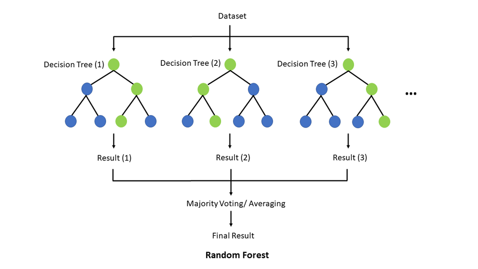
Many decision trees each give a prediction; the forest's prediction is the majority vote. (The figure feeds the same data to every tree; in a random forest each tree gets its own bootstrap sample.) Figure: TseKiChun (CC BY-SA 4.0), via Wikimedia Commons.
You use the forest straight from the library, through the same fit, predict and score as the
lines.
✏️ Your turn 5
On all nine oxides, does a forest beat the lines?
Why: a new model earns its place only with a better cross-validation score than the bar, 0.902, and its training score cannot tell you whether it does.
forest: aRandomForestClassifier(n_estimators=200, random_state=0)fitted onXandy.forest_train_score: its score on the same training rocks,Xandy.forest_scores: the five cross-validation scores of a new forest of the same kind, onXandy, andforest_cv, their mean.
Use these names, because the self-check looks for them: forest, forest_train_score and
forest_cv.
# ← your answer here: replace every ... with code
# nine_scores, nine_cv: the lines' five cross-validation scores and their mean, from Your turn 2
forest = RandomForestClassifier(n_estimators=200, random_state=0)
forest.fit(..., ...)                                  # the nine oxides and the setting of every training rock
forest_train_score = forest.score(..., ...)           # on the same rocks it learned from
forest_scores = cross_val_score(..., ..., ..., cv=5)  # the forest, then the nine oxides and the setting
forest_cv = np.mean(...)                              # the mean of the five scores
print("on the training rocks:", round(forest_train_score, 3))
print("cross-validation:", np.round(forest_scores, 3), " mean", round(forest_cv, 3))
print("the lines:       ", np.round(nine_scores, 3), " mean", round(nine_cv, 3))
# Self-check: run this after your answer. You do not need to read it — it only says whether something is off.
assert round(forest_train_score, 3) == 1.0, "fit the forest on X and y, then score it on X and y"
assert round(forest_cv, 3) == 0.931, "cross_val_score(forest, X, y, cv=5), then the mean"
print(f"✓ Your turn 5 — the forest scores {forest_train_score:.3f} on its training rocks and {forest_cv:.3f} by cross-validation")
1.000 on the training rocks, perfect again and again meaningless; 0.931 by cross-validation, above the lines' 0.902 on all 5 parts. On nine oxides the forest has more to work with, and it gains about 3 points.
Which oxides did the forest use? How much of a forest's decisions each column carried — the model's own account of what it used. Each question a tree asks makes its two sides less mixed; that gain is credited to the question's column, added up over all 200 trees, and scaled so the credits sum to 1.
importance = pd.Series(forest.feature_importances_, index=oxides).sort_values()
plt.figure(figsize=(7, 4))
plt.barh(importance.index, importance.values)
plt.xlabel("share of the credit")
plt.title("Which oxides the forest used (448 training rocks)")
plt.show()
Titanium first (0.321), then far less K2O (0.128) and SiO2 (0.119). Given all nine, the forest leans most on the element whose medians differed most clearly between the settings in section 1. Importance is not a law of nature: two columns that carry the same information share the credit. And potassium is also the oxide sea water changes most after a basalt erupts, so on old, altered sea floor, such as the Coast Ranges' slices, a geologist would lean on titanium rather than potassium.
5. Can a support vector machine beat them?
The widest gap. Of all the lines separating the two groups, take the one leaving the widest gap. Many lines can part two groups of rocks. The SVM picks the one that leaves the widest empty band between them, so a new rock has the most room to land on its own side. The rocks on the edge of the band, the support vectors, alone fix the line, which gives the method its name.
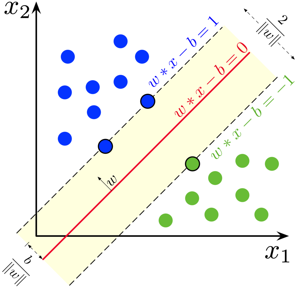
Two groups (blue, green) and the line that parts them (red) with the widest gap (yellow band); the circled points on the edge of the band are the support vectors. Figure: Larhmam (CC BY-SA 4.0), via Wikimedia Commons.
Real rocks overlap, so no band is empty: the SVM lets a few rocks sit inside the band, or even on
the wrong side, in exchange for a wider gap. With three settings, SVC finds a widest gap for
each pair (arc–ridge, arc–island, ridge–island), and the pairs vote. And plain SVC() may bend its
edges into curves to follow the clouds of rocks; the idea, the widest gap, is the same.
A gap is a distance, and a distance adds up the differences in each column in that column's own units. The oxides' standard deviations differ a lot:
oxide_spread = train[oxides].std()   # the standard deviation of each oxide, in weight percent
print(oxide_spread.round(2))
Magnesium, aluminium and silica vary by about 2 percent from rock to rock; manganese by 0.03, phosphorus by 0.22, potassium by 0.55. In raw units the distance is decided by the big oxides, and the small ones, potassium, phosphorus and manganese among them, barely count.
Scaling fixes this: from each column subtract its mean and divide by its standard deviation,
$$x_\text{scaled} = \frac{x - \text{mean}}{\text{std}}$$
so every column has mean 0 and spread 1. StandardScaler does it in two steps, like a model:
.fit(table) learns each column's mean and standard deviation, and .transform(table)
applies them. A simple case: 2 and 6 have mean 4 and standard deviation 2, so they become −1 and 1.
The mean and standard deviation are learned, like the model, from the training rows only. They are then used, unchanged, on the held-out rows. Scaling the held-out rows by their own mean would let the rocks we score on shape the model we score. The next cell makes one validation split of the training rocks, 358 to fit and 90 held out, and lets a scaler learn from the 358 only.
fit_rows, held_rows = train_test_split(train, test_size=0.2, random_state=0, stratify=train["setting"])
scaler = StandardScaler()
scaler.fit(fit_rows[oxides])           # learns each oxide's mean and standard deviation, from fit_rows only
learned = pd.DataFrame({"mean": scaler.mean_, "std": scaler.scale_}, index=oxides)
print(learned.round(3))
✏️ Your turn 6
Does the SVM do better on scaled columns?
Why: an SVM measures distance, so it needs scaled columns, and the scaling must be learned from the rows it fits on, then applied, unchanged, to the rows it is scored on.
fit_rows, held_rows and scaler come from the cell above. raw_score, an SVM on the raw oxides of
the same rows, is given.
fit_scaledandheld_scaled: the oxides offit_rowsand ofheld_rows, each through the samescaler'stransform.svm: anSVC()fitted onfit_scaledand the setting offit_rows.scaled_score: its score onheld_scaledand the setting ofheld_rows.
Use these names, because the self-check looks for them: raw_score and scaled_score.
# ← your answer here: replace every ... with code
raw_svm = SVC()
raw_svm.fit(fit_rows[oxides], fit_rows["setting"])
raw_score = raw_svm.score(held_rows[oxides], held_rows["setting"])
fit_scaled = scaler.transform(...)   # fit_rows' nine oxides
held_scaled = scaler.transform(...)  # held_rows' nine oxides, with the same scaler
svm = SVC()
svm.fit(..., ...)                    # the scaled training rows, and their setting
scaled_score = svm.score(..., ...)   # the scaled held-out rows, and their setting
print("SVM on the held-out rocks, raw columns:", round(raw_score, 3), "  scaled:", round(scaled_score, 3))
# Self-check: run this after your answer. You do not need to read it — it only says whether something is off.
assert round(raw_score, 3) == 0.811, "leave the given raw_score lines as they are"
assert round(scaled_score, 3) == 0.944, "scale both tables with the same scaler; fit on the scaled training rows, score on the scaled held-out rows"
print(f"✓ Your turn 6 — raw {raw_score:.3f}, scaled {scaled_score:.3f}")
From 0.811 to 0.944 on the same 90 rocks, by changing nothing but the units. To cross-validate the scaled SVM, those steps (learn the scaling, apply it, fit) must run again in every round, each time learning only from that round's four parts. Doing that by hand is easy to get wrong. A pipeline does it for you.
make_pipeline(StandardScaler(), SVC()) joins a scaler and an SVM into one model, pipe:
pipe.fit(table, labels)does both of your fitting lines: the scaler learns the mean and standard deviation oftableand scales it, then the SVM fits on the scaled rows;pipe.score(other, labels)andpipe.predict(other)scaleotherwith the stored mean and standard deviation, neverother's own, then score or predict;- given to
cross_val_score, the pipeline is fitted afresh in each round on that round's four parts, so every held-out part is scaled by what the other four learned.
The next cell checks the first two on your split: the pipeline's own scaler, pipe[0], learns the
same means as yours, and its score on held_rows is your scaled_score.
pipe = make_pipeline(StandardScaler(), SVC())             # step 0 scales, step 1 is the SVM
pipe.fit(fit_rows[oxides], fit_rows["setting"])           # the scaler learns from fit_rows, then the SVM fits
print("the pipeline's scaler learned:", pipe[0].mean_.round(2))
print("your scaler learned:          ", scaler.mean_.round(2))
pipe_score = pipe.score(held_rows[oxides], held_rows["setting"])    # held_rows is scaled with the stored mean and std
print("the pipeline on held_rows:", round(pipe_score, 3), "  yours:", round(scaled_score, 3))
✏️ Your turn 7
By cross-validation, does the scaled SVM beat the lines on nine oxides?
Why: one split can be lucky. The cross-validation mean is what every model is judged by, against the bar of 0.902.
svm_raw_scores: the five cross-validation scores of a plainSVC()onXandy.svm_nine: the pipelinemake_pipeline(StandardScaler(), SVC()), fitted onXandy. You will use it again at the end.svm_scores: the five cross-validation scores ofsvm_nineonXandy.svm_raw_cvandsvm_cv: the two means.
Use these names, because the self-check looks for them: svm_raw_cv and svm_cv.
# ← your answer here: replace every ... with code
# nine_cv: the lines' cross-validation mean on nine oxides, from Your turn 2
svm_raw_scores = cross_val_score(..., ..., ..., cv=5)  # a plain SVM, then the nine oxides and the setting
svm_nine = ...                                         # the pipeline: scale, then an SVM
svm_nine.fit(..., ...)                                 # all training rocks: the nine oxides, and the setting
svm_scores = cross_val_score(..., ..., ..., cv=5)      # svm_nine, then the same rocks
svm_raw_cv = np.mean(...)                              # the mean of the raw SVM's five scores
svm_cv = np.mean(...)                                  # the mean of the pipeline's five scores
print("SVM by cross-validation, raw:", round(svm_raw_cv, 3), "  scaled in a pipeline:", round(svm_cv, 3))
print("the lines:", round(nine_cv, 3))
# Self-check: run this after your answer. You do not need to read it — it only says whether something is off.
assert round(svm_raw_cv, 3) == 0.794, "a plain SVC() on X and y, cv=5, then the mean"
assert round(svm_cv, 3) == 0.931, "make_pipeline(StandardScaler(), SVC()) on X and y, cv=5, then the mean"
print(f"✓ Your turn 7 — SVM raw {svm_raw_cv:.3f}, scaled {svm_cv:.3f}")
0.794 raw, below the lines' 0.902; 0.931 scaled in a pipeline, above them. The SVM is strong once its columns are scaled, and poor without it.
The question, answered
Three classifiers compared, and the sealed rocks opened once
Three classifiers, one interface. The lines, the forest and the SVM were each made, fitted and
scored with the same three calls, fit, predict and score, so trying another model was one line.
What differs is the boundary each draws. Here are their regions on titanium and potassium, side by
side:
forest_tk = RandomForestClassifier(n_estimators=200, random_state=0).fit(train[ti_k], y)   # a forest on Ti and K
svm_tk = make_pipeline(StandardScaler(), SVC()).fit(train[ti_k], y)                     # a scaled SVM on Ti and K
plt.figure(figsize=(16, 4.5))
plt.subplot(1, 3, 1)                # three panels in a row: this is the first
draw_regions(line_tk, "Logistic regression: straight edges")
plt.subplot(1, 3, 2)
draw_regions(forest_tk, "Random forest: boxes")
plt.subplot(1, 3, 3)
draw_regions(svm_tk, "SVM: smooth curves")
plt.show()
forest_tk_cv = np.mean(cross_val_score(forest_tk, train[ti_k], y, cv=5))
svm_tk_cv = np.mean(cross_val_score(svm_tk, train[ti_k], y, cv=5))
print("cross-validation on Ti and K: lines", round(np.mean(tk_scores), 3), "  forest", round(forest_tk_cv, 3), "  SVM", round(svm_tk_cv, 3))
Straight edges, boxes, smooth curves: three ways to cut the same map. The next cell lines up the four cross-validation means and spreads.
print("lines on Ti and K:    mean", round(np.mean(tk_scores), 5),   # five decimals, to show the tie below
      "  spread", round(np.std(tk_scores), 3))
print("lines on nine oxides: mean", round(np.mean(nine_scores), 5), "  spread", round(np.std(nine_scores), 3))
print("forest:               mean", round(np.mean(forest_scores), 5), "  spread", round(np.std(forest_scores), 3))
print("SVM, scaled:          mean", round(np.mean(svm_scores), 5), "  spread", round(np.std(svm_scores), 3))
The forest and the scaled SVM tie exactly, 0.931 each (they get the same number of rocks right in all), and both beat last week's lines (0.902). On two columns the flexible models gained little or nothing: the forest lost a little (0.862 against 0.868), and the scaled SVM gained about one rock in a hundred (0.877), less than the spread of the five scores. So which method wins depends on the data, and it is decided by cross-validation, not by reputation.
Now the sealed rocks, which no model and no decision has touched. Every model is fitted on all the training rocks and scored on them once: does what cross-validation concluded hold on rocks no model has ever seen?
✏️ Your turn 8
Does the cross-validation ranking hold on the sealed rocks?
Why: cross-validation is only worth trusting if its conclusions carry over to new rocks, and the sealed rocks are the one check on that.
Every model was fitted once, on all 448 training rocks: line_tk in Your turn 1,
line_nine in section 2, forest in Your turn 5 and svm_nine in Your turn 7. Now each is scored
once on the sealed rocks.
sealed_lines_tk,sealed_lines_nine,sealed_forestandsealed_svm: each model's score on the sealed rocks, on the columns it was fitted on.
The given lines print each sealed score beside its cross-validation mean.
Use these names, because the self-check looks for them: sealed_lines_tk, sealed_lines_nine,
sealed_forest and sealed_svm.
# ← your answer here: replace every ... with code
# line_tk, line_nine, forest, svm_nine: fitted on all training rocks; sealed: the 192 sealed rocks
sealed_lines_tk = line_tk.score(..., ...)      # the sealed rocks: TiO2 and K2O, and their setting
sealed_lines_nine = line_nine.score(..., ...)  # the sealed rocks: the nine oxides, and their setting
sealed_forest = forest.score(..., ...)         # the same
sealed_svm = svm_nine.score(..., ...)          # the same

print("lines on Ti and K:     cross-validation", round(np.mean(tk_scores), 3), "  sealed", round(sealed_lines_tk, 3))
print("lines on nine oxides:  cross-validation", round(np.mean(nine_scores), 3), "  sealed", round(sealed_lines_nine, 3))
print("forest:                cross-validation", round(np.mean(forest_scores), 3), "  sealed", round(sealed_forest, 3))
print("SVM, scaled:           cross-validation", round(np.mean(svm_scores), 3), "  sealed", round(sealed_svm, 3))
# Self-check: run this after your answer. You do not need to read it — it only says whether something is off.
SA = {'lines, Ti and K': 0.854, 'lines, nine oxides': 0.911, 'forest': 0.948, 'SVM, scaled': 0.953}
assert round(sealed_lines_tk, 3) == SA["lines, Ti and K"], "line_tk.score(sealed[ti_k], sealed['setting'])"
assert round(sealed_lines_nine, 3) == SA["lines, nine oxides"], "line_nine.score(sealed[oxides], sealed['setting'])"
assert round(sealed_forest, 3) == SA["forest"], "forest.score(sealed[oxides], sealed['setting'])"
assert round(sealed_svm, 3) == SA["SVM, scaled"], "svm_nine.score(sealed[oxides], sealed['setting'])"
print(f"✓ Your turn 8 — the forest {sealed_forest:.3f} and the SVM {sealed_svm:.3f} on the sealed rocks")
The ranking holds, as far as these rocks can tell. On the sealed rocks the lines on titanium and potassium score 0.854, the lines on nine oxides 0.911, and the two flexible models 0.948 (forest) and 0.953 (SVM): the same order cross-validation found, each close to its cross-validation mean. Guessing the commonest setting gets 0.354 of the sealed rocks right.
The conclusion is not "the best model is X". Two things are clear: nine oxides beat titanium and potassium, and on nine oxides the forest and the SVM both beat last week's lines. Between the forest and the SVM the rocks cannot decide: they tied exactly on the five parts, and on the sealed rocks they differ by 1 rock of 192. Picking one by its last decimal would be reading noise. Either one, used on new rocks from this compilation, should name the setting about 19 times in 20.
The answer: from its chemistry. For rocks like these, a forest or an SVM on nine oxides predicts
the setting of about 19 in 20 rocks it never saw (0.948 and
0.953). Titanium carries the most, the one oxide whose medians put all three settings in order, as section 1 showed and
the forest's importance confirmed. Training scores said nothing (the forest's was
1.000); cross-validation told the models apart, and the sealed rocks confirmed what
it found. The three classifiers share fit, predict and score, so all three were tried: on nine
oxides the flexible ones gained a little over the lines, and on two elements little or nothing. Which method
wins depends on the data, and on these rocks two methods are equally good.
Three classifiers, side by side
| Logistic regression (the lines) | Random forest | Support vector machine (SVM) | |
|---|---|---|---|
| How it predicts a setting | one weighted sum per setting, turned into probabilities; the largest wins | a vote of 200 decision trees | the side of the widest gap between each pair of settings |
| Its boundary on Ti and K | straight edges | boxes | smooth curves |
| Strength | simple, readable weights; the bar to beat | bends to the data; columns in any units; feature importance | strong once its columns are scaled |
| Weakness | cannot bend | overfits its training rocks (1.000); not one readable rule | poor on unscaled columns |
| Cross-validation, Ti and K | 0.868 | 0.862 | 0.877 |
| Cross-validation, nine oxides | 0.902 | 0.931 | 0.931 (scaled) |
Which to use: start with the lines, the bar to beat. Keep a flexible model only if its cross-validation score beats the bar. Whichever you pick, test it once.
Week 10 summary
The science
Where was this basalt made?
A basalt's chemistry records where it formed. Its big oxides (silica about 50 percent, Al2O3, CaO, MgO, Na2O) build its minerals and barely differ between settings; three small ones differ a lot: P2O5 2.9 times, TiO2 3.1 times and K2O 5.9 times from the lowest setting median to the highest. They fit badly in mantle minerals and gather in the melt, so how much the mantle melts, and whether water from a sinking plate is present, sets how much of them a basalt holds. A training score is not the model's score. Training, validation and test sets each have one job: the training rocks fit, the validation rocks compare, and the test rocks, touched by no decision, check once whether the comparison holds. A forest scores 1.000 on the rocks it learned from and less on rocks held out. Cross-validation chooses the model: five parts, each held out once, give a fair score and its spread (cross_val_score, cv=5). One validation split moved the same model's score from 0.867 to 0.967. Three classifiers, compared. Logistic regression, the random forest and the SVM share fit, predict and score, so trying another is one line. Logistic regression draws straight edges: simple and readable, the model to beat, but it cannot bend. A random forest bends to the data and takes columns in any units, but cannot be read as one rule. An SVM draws smooth curves and needs scaled columns. On nine oxides the flexible models gain a little (0.931 each against 0.902); on titanium and potassium they gain little or nothing (forest 0.862, scaled SVM 0.877, against 0.868 for the lines). The method is chosen by cross-validation, not by reputation.
- Tectonic settings of basalt. Basalt is made in three places, where the mantle melts: where two plates pull apart (a mid-ocean ridge), where one plate sinks under another (an island arc), and over a hot plume, usually far from any plate edge (an ocean island).
- Major oxide, trace element. A rock analysis gives the common elements as oxides, in percent of the rock's weight (SiO2, TiO2), and the rare ones in parts per million (V, Sr).
- Feature importance. How much of a forest's decisions each column carried — the model's own account of what it used.
- Cross-validation. Cut the rows into five parts; hold out each part in turn, train on the other four, and score on the one held out. Five scores, and every row tested once.
- Decision tree. A flowchart of yes/no questions, learned from the data instead of written by hand.
- Random forest. Ask many slightly different trees and take a vote.
- SVM. Of all the lines separating the two groups, take the one leaving the widest gap.
The code
| Function | What it does |
|---|---|
| Python | |
ConfusionMatrixDisplay(counts, display_labels=names).plot() |
draw a confusion matrix as a grid shaded by count, true labels down the side, predictions along the bottom |
make_pipeline(StandardScaler(), SVC()) |
one model that scales the columns and then fits; inside cross-validation each part learns its own scaling |
cross_val_score(model, X, y, cv=5) |
hold out each of five parts in turn, fit a new copy of the model on the other four, and return the five held-out scores |
len(table) |
how many rows |
for x in things: |
do the same thing once for each item |
list.append(x) |
add one item to the end of a list |
| NumPy | |
np.mean(values) / np.std(values) |
the average and the standard deviation of a list or an array |
np.argmax(values) / np.argmin(values) |
the position of the largest / smallest value, to read the same position out of another array or list |
| Matplotlib | |
plt.plot(x, y) |
join points with a line |
| scikit-learn | |
RandomForestClassifier(n_estimators=200, random_state=0) |
many slightly different trees, voting |
SVC() |
the widest-gap classifier; give it scaled columns or the gap means nothing |
StandardScaler() |
put every column on the same footing, so a distance across them means something |
scaler.fit(table) / scaler.transform(table) |
learn each column's mean and standard deviation from the training rows, then scale any rows with those same numbers |
forest.feature_importances_ |
one number per column: how much of the forest's decisions it carried |
model.fit(X_train, y_train) |
learn from the training rows |
LogisticRegression() |
draw the straight line that best separates two labelled groups; with three labels, one weighted sum per label, the edges where two sums tie |
confusion_matrix(y, pred) |
count right and wrong predictions: true settings down the side, predictions across, the right ones on the diagonal |
model.fit(X, y) / model.predict(X) |
learn from the training rows, then predict for any rows |
Homework
What the homework practises, each with the class Your turn to look back at:
- comparing models by cross-validation (Your turns 2 and 3);
- a training score against a cross-validation score (Your turns 4 and 5);
- the SVM in a pipeline (Your turn 7);
- checking on sealed rocks whether the cross-validation ranking holds (Your turn 8).
It has three parts, each a step of class on new rocks, with less given.
- Part 1 (Your turn 9): which two elements should a geologist measure, if only two: titanium and vanadium, the pair of a famous diagram from 1982, or titanium and strontium?
- Part 2 (Your turns 10 and 11): on the better pair, do the forest or the SVM beat the lines? Then does their cross-validation ranking hold on the sealed rocks?
- Part 3 (Your turn 12): would the three models work on rocks from a different compilation?
The next cell remakes what the homework reads. After a restart, run the Setup cell at the top first, then this one.
# ── Checkpoint ── run this if you restarted the kernel or fell behind ──
rocks = pd.read_csv(CACHE + "/week10_vermeesch_basalts.csv")   # the basalts again, read and fixed as in Setup
rocks = rocks.rename(columns={"affinity": "setting", "P2O5(wt%)": "P2O5_wt_percent"})
rocks.loc[rocks["MnO_wt_percent"] > 5, "MnO_wt_percent"] = np.nan
oxides = ["SiO2_wt_percent", "TiO2_wt_percent", "Al2O3_wt_percent", "CaO_wt_percent", "MgO_wt_percent",
          "MnO_wt_percent", "K2O_wt_percent", "Na2O_wt_percent", "P2O5_wt_percent"]
rocks_ox = rocks.dropna(subset=oxides)   # all nine oxides, for part 3
print(len(rocks_ox), "rocks with all nine oxides")
Part 1: titanium and vanadium, or titanium and strontium?
Two trace elements. Vanadium and strontium are measured in parts per million. 494 rocks in the file have titanium, vanadium and strontium all measured (180 ridge, 158 arc and 156 ocean-island rocks). As in class, the next cell seals 30 percent of them first, and every look from here on uses the training rocks.
rocks_trace = rocks.dropna(subset=["TiO2_wt_percent", "V_ppm", "Sr_ppm"])   # rocks with titanium, vanadium and strontium
train_trace, sealed_trace = train_test_split(rocks_trace, test_size=0.3, random_state=0, stratify=rocks_trace["setting"])
ti_and_v = ["TiO2_wt_percent", "V_ppm"]     # the names of the titanium and vanadium columns
ti_and_sr = ["TiO2_wt_percent", "Sr_ppm"]   # the names of the titanium and strontium columns
print(len(train_trace), "training rocks,", len(sealed_trace), "sealed")
Lines drawn by hand: Shervais's diagram. In 1982 the geologist John Shervais plotted titanium against vanadium. Vanadium alone barely differs between the settings (median 280, 271 and 274 ppm in the arc, ridge and island training rocks). Shervais used it as a ruler. As a melt cools and grows crystals, vanadium and titanium change together, so their ratio, Ti/V, changes less than either and keeps the mark of the melting. And an arc's melt is wet and oxidised, which lets more vanadium into it, so arc basalt holds much vanadium for its titanium. He drew two lines, at Ti/V = 20 and Ti/V = 50: arc rocks below 20, ridge rocks between, ocean islands above 50. (That last field is for the alkaline ocean-island basalts; island tholeiites, like most of Hawaii's lava, plot between 20 and 50 with the ridges.)
Titanium is reported as TiO2 in weight percent. Titanium is 47.87 of TiO2's 79.87 units of mass (their atomic masses), so 1 percent TiO2 holds 10,000 × 47.87 / 79.87 ≈ 5993 parts per million of titanium. The next cell draws the training rocks with his two lines and scores his rule.
ti_v_ratio = train_trace["TiO2_wt_percent"] * 5993 / train_trace["V_ppm"]   # Ti in ppm, over V in ppm
shervais = []
for r in ti_v_ratio:
    if r < 20:
        shervais.append("IAB")
    elif r < 50:
        shervais.append("MORB")
    else:
        shervais.append("OIB")
right = (np.array(shervais) == train_trace["setting"]).sum()
print("Shervais's lines:", right, "of", len(train_trace), "training rocks right =", round(right / len(train_trace), 3))

plt.figure(figsize=(7, 4.5))
for setting, marker in [("IAB", "o"), ("MORB", "s"), ("OIB", "^")]:
    some = train_trace[train_trace["setting"] == setting]
    plt.scatter(some["TiO2_wt_percent"], some["V_ppm"], s=12, marker=marker, label=setting)
tio2 = np.arange(0, 5.01, 0.1)
for ratio in [20, 50]:
    plt.plot(tio2, tio2 * 5993 / ratio, color="black", lw=1)   # V = Ti / ratio
plt.text(1.2, 660, "Ti/V = 20")
plt.text(4.25, 450, "Ti/V = 50")
plt.xlim(0, 5)
plt.ylim(0, 700)
plt.xlabel("TiO2 (weight percent)")
plt.ylabel("V (parts per million)")
plt.title("Shervais's lines, drawn by hand in 1982 (" + str(len(train_trace)) + " training rocks)")
plt.legend()
plt.show()
270 of 345 right (0.783), from two lines a person drew. 24 of the island rocks fall between the lines, where Shervais put the ridges. A model can draw its own lines, and strontium is another candidate partner for titanium. Arc melts are richer in it than ridge melts: the water rising from the sinking plate carries it into the melt, as it carries potassium.
✏️ Your turn 9 (homework part 1)
Which pair predicts the setting better on rocks held out: titanium and vanadium, or titanium and strontium?
Why: a geologist with money for two measurements wants the pair that generalizes best. Both pairs are scored on the same training rocks, so the comparison is fair. This repeats Your turn 3.
tv_scores: the five cross-validation scores of aLogisticRegression(max_iter=5000)ontrain_trace's titanium and vanadium (ti_and_v) and its setting, five parts.sr_scores: the same for titanium and strontium (ti_and_sr).tv_cvandsr_cv: their means.
The prints are given.
Use these names, because the self-check looks for them: tv_cv and sr_cv.
# ← your answer here: replace every ... with code
tv_lines = ...                                         # last week's lines: logistic regression, max_iter 5000
tv_scores = cross_val_score(tv_lines, ..., ..., cv=5)  # the training rocks' TiO2 and V, and their setting
sr_lines = ...                                         # a new model of the same kind
sr_scores = cross_val_score(sr_lines, ..., ..., cv=5)  # the training rocks' TiO2 and Sr, and their setting
tv_cv = np.mean(...)                                   # the five Ti-V scores
sr_cv = np.mean(...)                                   # the five Ti-Sr scores
print("Ti and V: ", np.round(tv_scores, 3), " mean", round(tv_cv, 3))
print("Ti and Sr:", np.round(sr_scores, 3), " mean", round(sr_cv, 3))
# Self-check: run this after your answer. You do not need to read it — it only says whether something is off.
assert round(tv_cv, 3) == 0.835, "the lines on train_trace[ti_and_v] and train_trace['setting'], cv=5, then the mean"
assert round(sr_cv, 3) == 0.910, "the lines on train_trace[ti_and_sr] and train_trace['setting'], cv=5, then the mean"
print(f"✓ Your turn 9 — Ti and V {tv_cv:.3f}, Ti and Sr {sr_cv:.3f}")
What the numbers mean. Which pair scores higher, and does it win on every part or only on average? Why might strontium part arcs from ridges (think of the arc's water)? Then: sea water moves strontium in and out of a basalt after it erupts, while titanium and vanadium stay put. What can a score on these rocks, whose alteration nobody recorded, not tell you about old, altered sea floor?
✏️ Your turn 10 (homework part 2, the models)
On titanium and strontium, do the forest and the SVM beat the lines?
Why: in class, on nine oxides, the forest and the scaled SVM beat the lines. Does that hold on two columns? And strontium is counted in hundreds of parts per million, titanium in a few percent: does the SVM notice? This repeats Your turns 5 and 7.
All on train_trace's titanium and strontium (ti_and_sr) and its setting, with cv=5:
forest_sr: a forest like the class's, fitted on the training rocks;forest_sr_train: its score on those same rocks.forest_sr_scores: the five cross-validation scores of a new forest of the same kind.svm_raw_sr_scores: the five cross-validation scores of a plainSVC()on the raw columns.svm_sr_scores: the same for a pipeline that scales and then fits an SVM.
The prints, with each column's standard deviation, are given.
Use these names, because the self-check looks for them: forest_sr_train, forest_sr_scores,
svm_raw_sr_scores and svm_sr_scores.
# ← your answer here: replace every ... with code
forest_sr = ...                                                    # a forest of 200 trees, random_state 0
forest_sr.fit(..., ...)                                            # the training rocks' TiO2 and Sr, and their setting
forest_sr_train = forest_sr.score(..., ...)                        # the same training rocks
forest_sr_scores = cross_val_score(forest_sr, ..., ..., cv=5)      # TiO2 and Sr, and the setting
plain_svm_sr = ...                                                 # a plain SVM
svm_raw_sr_scores = cross_val_score(plain_svm_sr, ..., ..., cv=5)  # TiO2 and Sr, and the setting
scaled_svm_sr = ...                                                # a pipeline: scale, then an SVM
scaled_svm_sr.fit(..., ...)                                        # the training rocks' TiO2 and Sr, and their setting
svm_sr_scores = cross_val_score(scaled_svm_sr, ..., ..., cv=5)     # TiO2 and Sr, and the setting
print("forest: on its training rocks", round(forest_sr_train, 3), "  cross-validation", round(np.mean(forest_sr_scores), 3))
print("SVM: raw", round(np.mean(svm_raw_sr_scores), 3), "  scaled in a pipeline", round(np.mean(svm_sr_scores), 3))
sr_columns_spread = train_trace[ti_and_sr].std()
print(sr_columns_spread.round(2))
# Self-check: run this after your answer. You do not need to read it — it only says whether something is off.
assert round(forest_sr_train, 3) == 1.000, "the forest scored on the same training rocks it was fitted on"
assert round(np.mean(forest_sr_scores), 3) == 0.904, "a new forest of 200 trees, random_state=0, on train_trace[ti_and_sr], cv=5"
assert round(np.mean(svm_raw_sr_scores), 3) == 0.678, "a plain SVC() on the raw columns, cv=5"
assert round(np.mean(svm_sr_scores), 3) == 0.913, "make_pipeline(StandardScaler(), SVC()), cv=5"
print(f"✓ Your turn 10 — forest {np.mean(forest_sr_scores):.3f}, SVM raw {np.mean(svm_raw_sr_scores):.3f}, scaled {np.mean(svm_sr_scores):.3f}")
What the numbers mean. How far apart are the forest's training score and its cross-validation score, and which one tells you about new rocks? How much does scaling change the SVM? Compare the two standard deviations: in raw units, which element decides the size of the gap?
✏️ Your turn 11 (homework part 2, the sealed rocks)
Does the cross-validation ranking hold on the sealed rocks?
Why: this is Your turn 8 on your own. Each model is fitted on all the training rocks and scored once on the sealed rocks, beside its cross-validation mean.
forest_sr and scaled_svm_sr were fitted in Your turn 10. sr_lines, from Your turn 9, was only
cross-validated, so fit it once first.
hw_sealed_lines,hw_sealed_forestandhw_sealed_svm: each model's score onsealed_trace's titanium and strontium and its setting.
The given lines print each sealed score beside its cross-validation mean.
Use these names, because the self-check looks for them: hw_sealed_lines, hw_sealed_forest
and hw_sealed_svm.
# ← your answer here: replace every ... with code
# sr_lines, sr_scores: Your turn 9; forest_sr, scaled_svm_sr, forest_sr_scores, svm_sr_scores: Your turn 10
sr_lines.fit(..., ...)                         # all training rocks: TiO2 and Sr, and their setting
hw_sealed_lines = sr_lines.score(..., ...)     # the sealed rocks: TiO2 and Sr, and their setting
hw_sealed_forest = forest_sr.score(..., ...)   # the same
hw_sealed_svm = scaled_svm_sr.score(..., ...)  # the same

print("lines:  cross-validation", round(np.mean(sr_scores), 3), "  sealed", round(hw_sealed_lines, 3))
print("forest: cross-validation", round(np.mean(forest_sr_scores), 3), "  sealed", round(hw_sealed_forest, 3))
print("SVM:    cross-validation", round(np.mean(svm_sr_scores), 3), "  sealed", round(hw_sealed_svm, 3))
# Self-check: run this after your answer. You do not need to read it — it only says whether something is off.
assert round(hw_sealed_lines, 3) == 0.94, "sr_lines.fit on train_trace[ti_and_sr]; score on sealed_trace[ti_and_sr]"
assert round(hw_sealed_forest, 3) == 0.933, "forest_sr.score(sealed_trace[ti_and_sr], sealed_trace['setting'])"
assert round(hw_sealed_svm, 3) == 0.946, "scaled_svm_sr.score(sealed_trace[ti_and_sr], sealed_trace['setting'])"
print(f"✓ Your turn 11 — lines {hw_sealed_lines:.3f}, forest {hw_sealed_forest:.3f}, SVM {hw_sealed_svm:.3f} on the sealed rocks")
What the numbers mean. Do the three models keep the same order on the sealed rocks as by cross-validation? Are the differences large compared with the spread of each model's five cross-validation scores? When does a flexible model, a forest or an SVM, pay for itself?
Rocks from somewhere else
The sealed rocks came from Vermeesch's own compilation, and rocks from one volcano can sit on both sides of a split. In 2022 the geologist Luc Doucet and colleagues compiled a much larger set of basalts of known setting, from two online databases (EarthChem and GEOROC), kept to rocks in the basalt silica range (43 to 53 percent silica, sodium plus potassium oxides below 5 percent; the rocks read here run from 45 to 53). The next cell reads 2,400 of their rocks, 800 per setting, with the same nine oxides and where each came from: a place, or for every ridge rock, PetDB, a database of ridge rocks from around the world.
# Doucet et al. (2022), Earth-Science Reviews 233, 104192, Supplementary Table S1:
# 800 rocks per setting, with all nine oxides (ARC-O, their oceanic arcs, renamed IAB).
doucet = pd.read_csv(CACHE + "/week10_doucet2022_basalts.csv")
print(list(doucet.columns))   # the same nine oxide names as class
print(doucet.groupby("setting")["location"].value_counts())
✏️ Your turn 12 (homework part 3)
Would the three models work on rocks from somewhere else?
Why: a test on rocks from the same compilation says how a model does on rocks like those. Doucet's rocks were gathered by other people, by other rules, and every arc rock is from Izu-Bonin. This repeats Your turn 8 with a new test set.
The test is now Doucet's rocks, so each model may learn from all 640 Vermeesch rocks with
nine oxides (rocks_ox, from the checkpoint: the class's training and sealed rocks together).
doucet_lines: last week's lines, fitted onrocks_ox's nine oxides and setting, scored ondoucet's nine oxides and setting.doucet_forest: the same for a forest like the class's.doucet_svm: the same for the pipeline that scales and then fits an SVM.
The given lines print each score beside the same model's score on the class's sealed rocks.
Use these names, because the self-check looks for them: doucet_lines, doucet_forest and
doucet_svm.
# ← your answer here: replace every ... with code
# rocks_ox: the 640 Vermeesch rocks with all nine oxides; doucet: Doucet's 2,400 rocks
lines_all = ...                           # last week's lines: logistic regression, max_iter 5000
lines_all.fit(..., ...)                   # rocks_ox's nine oxides, and their setting
doucet_lines = lines_all.score(..., ...)  # Doucet's nine oxides, and their setting

forest_all = ...                            # a forest of 200 trees, random_state 0
forest_all.fit(..., ...)                    # rocks_ox's nine oxides, and their setting
doucet_forest = forest_all.score(..., ...)  # Doucet's nine oxides, and their setting

svm_all = ...                         # a pipeline: scale, then an SVM
svm_all.fit(..., ...)                 # rocks_ox's nine oxides, and their setting
doucet_svm = svm_all.score(..., ...)  # Doucet's nine oxides, and their setting

print("lines:  Doucet", round(doucet_lines, 3), "  class sealed rocks 0.911")
print("forest: Doucet", round(doucet_forest, 3), "  class sealed rocks 0.948")
print("SVM:    Doucet", round(doucet_svm, 3), "  class sealed rocks 0.953")
# Self-check: run this after your answer. You do not need to read it — it only says whether something is off.
assert round(doucet_lines, 3) == 0.749, "the lines fitted on rocks_ox's nine oxides and setting, scored on doucet's"
assert round(doucet_forest, 3) == 0.869, "a forest of 200 trees, random_state=0, fitted on rocks_ox, scored on doucet"
assert round(doucet_svm, 3) == 0.854, "the pipeline fitted on rocks_ox's nine oxides and setting, scored on doucet's"
print(f"✓ Your turn 12 — lines {doucet_lines:.3f}, forest {doucet_forest:.3f}, SVM {doucet_svm:.3f} on Doucet's rocks")
What the numbers mean. How far does each model's score fall from its score on the class's sealed rocks? Does the order of the three models stay the same? Where do Doucet's rocks of each setting come from, and how might rocks from a few places differ from Vermeesch's worldwide mix? What does that say about the scores you found in class?