Record monthly warmth in the Pacific: is a record El Niño coming, and how far ahead can we forecast it?¶

EPS 88 · PyEarth · final project. Open your own copy on DataHub: click here.

In October 2026 the sea surface in the middle of the tropical Pacific was 3.25 °C warmer than usual for the month, the largest excess for any month in NOAA's satellite-era record, which starts in 1982 (the previous largest was +2.72 °C, in November 2015). A strong El Niño is under way. Is it a record? Not yet by NOAA's official measure, the Oceanic Niño Index, which averages three months: for August 2026 to October 2026 it stood at +2.46 °C, below the record +2.59 °C of November 2015 to January 2016 (the index starts in 1950). The coming winter decides. El Niño shifts rain and drought around the world, so forecasters try to see it coming months ahead. In this project you build a forecast of the Pacific's temperature three months ahead and test it on years it has never seen. The leaderboard scores your forecasts for 2018 to 2025, which your file leaves blank, and ranks everyone's entries.

This notebook is built like a weekly notebook: a few questions lead it, each section answers one, and every place you work opens with a pencil icon ✏️ and the words Your turn. The difference is how much you write. Each Your turn says why the step matters and gives a numbered plan in words; the cell under it is empty, and you write all of the code, looking back at the weekly notebook it names. A self-check cell follows. Run it: it tells you whether your numbers are right, as in every week.

The last Your turn is your leaderboard entry: it saves the file submission.csv. Run every cell so your answers and figures are saved in the file, then download this notebook itself — the .ipynb file — and upload it to Gradescope together with submission.csv. In JupyterLab: File ▸ Download, or right-click the file in the left-hand panel and choose Download. The leaderboard scores your file on answers you never see and ranks everyone's entries.

Two habits from the first minute. A cell runs when you press Shift+Enter, and the notebook remembers everything it has already run — so when something breaks and you cannot see why, Kernel → Restart Kernel and Run All Cells throws the memory away and rebuilds it from the top. That is never the wrong thing to do.

What you'll be able to do¶

The science. Say what El Niño is and how it is measured, why an anomaly that appears in summer tends to grow while one in spring tends to fade, and how warm water stored along the equator can warn of an El Niño months ahead.

The code. You write every line: a groupby and a ranking, a function for the typical miss, .shift to line up each month with the month three later, a loop over forecast leads, a split by time, LinearRegression one start month at a time, a function that makes those forecasts, a paired bootstrap over whole years, and a submission.csv table.

The four questions of the project:

1. How strong is this El Niño compared with every one since 1982?
2. How far ahead does "the same as now" work?
3. Does a fitted line do better, and why does the start month matter?
4. Does the ocean's stored heat help, and in every decade?

What you hand in, and when¶

One Gradescope assignment, "Final project: El Niño", takes everything.

• Individual work. Start now; Gradescope takes uploads from Wed 25 Nov, and the project is due Wed 16 Dec. Mon 7 Dec (RRR week) has no class, but you are welcome to come to the room in class time and work on your notebook.
• Every upload carries two files: submission.csv (your leaderboard entry, made by the last Your turn) and this notebook. Gradescope cannot check this for you, so follow these steps:
  1. In DataHub, save the notebook (File ▸ Save). submission.csv is in the same folder as the notebook, in the left-hand panel.
  2. Download both: right-click each file in the left-hand panel and choose Download.
  3. In Gradescope, open Final project: El Niño, click Upload Submission, and select both files (hold Ctrl, or Cmd on a Mac, to select the second), or drag both into the window. Type a name for the leaderboard: your own name or a nickname. Your classmates will see it next to your score.
  4. Check that Gradescope lists both files, then upload. If the result says a file is missing, upload both again.
• Up to 10 uploads that change submission.csv are scored on the leaderboard. An upload that changes only the notebook is free.
• Everything is due Wed 16 Dec at 23:59 Pacific time: the notebook and your last entry.
• Before every upload: Kernel → Restart Kernel and Run All Cells must run from top to bottom without an error.

How it is graded (100 points). The Your turns are graded like a week's. The leaderboard gives two grades: one for a valid entry that beats forecasting zero, and one for your rank, on the final score from the hidden part of the board. Choose your entry by your own fair tests, not by the public score.

What	Points	Graded by	Full marks when
Your turns 1 to 10	80	Gradescope, when you upload	each Your turn by its self-check, and the notebook runs from top to bottom without an error
Leaderboard entry	10	Gradescope, pass or fail	your last submission.csv is valid and its final score beats forecasting an anomaly of zero for every month
Leaderboard rank	10	after the board closes	your final score, on the hidden part, ranked among the students on this project: top quarter 10, second quarter 8, third quarter 6, last quarter 4; a tie takes the higher band; no valid entry 0

Setup¶

Run the next two cells once. All their code is given. Two files ship with the course:

• trackT15_enso_monthly.csv: one row per month from January 1982. nino34 is the sea-surface temperature anomaly in the Niño 3.4 box, in °C, from NOAA's Climate Prediction Center; wwv is the warm water volume anomaly, from NOAA's Pacific Marine Environmental Laboratory (PMEL), in units of 10¹⁴ m³. Section 1 and section 4 explain each.
• trackT15_submission_template.csv: the empty submission template, the table the leaderboard reads.

In [ ]:

import numpy as np
from sklearn.linear_model import LinearRegression
import pandas as pd
import matplotlib.pyplot as plt

# house style, set once, so every plot cell below holds only what matters
plt.rcParams.update({"figure.figsize": (8, 4), "figure.dpi": 110,
                     "axes.grid": True, "grid.alpha": 0.3, "axes.axisbelow": True})

CACHE = "https://raw.githubusercontent.com/AI4EPS/EPS88_PyEarth/main/data"

enso = pd.read_csv(CACHE + "/trackT15_enso_monthly.csv")
template = pd.read_csv(CACHE + "/trackT15_submission_template.csv")
print("monthly file:", enso.shape, "  template:", template.shape)

import numpy as np from sklearn.linear_model import LinearRegression import pandas as pd import matplotlib.pyplot as plt # house style, set once, so every plot cell below holds only what matters plt.rcParams.update({"figure.figsize": (8, 4), "figure.dpi": 110, "axes.grid": True, "grid.alpha": 0.3, "axes.axisbelow": True}) CACHE = "https://raw.githubusercontent.com/AI4EPS/EPS88_PyEarth/main/data" enso = pd.read_csv(CACHE + "/trackT15_enso_monthly.csv") template = pd.read_csv(CACHE + "/trackT15_submission_template.csv") print("monthly file:", enso.shape, " template:", template.shape)

The next cell adds a time column for plotting, the year as a decimal, and counts the blank months. The months from January 2018 to October 2025 are blank on purpose: they are the leaderboard's hidden answers. Each row is still there, so the rows stay one month apart.

In [ ]:

enso["time"] = enso["year"] + (enso["month"] - 1) / 12

blank = enso["nino34"].isna()
print("months:", len(enso), "  blank:", blank.sum(), "  with a value:", (~blank).sum())
print(enso.tail(3))

enso["time"] = enso["year"] + (enso["month"] - 1) / 12 blank = enso["nino34"].isna() print("months:", len(enso), " blank:", blank.sum(), " with a value:", (~blank).sum()) print(enso.tail(3))

1. How strong is this El Niño compared with every one since 1982?¶

El Niño is a warming of the surface of the central and eastern tropical Pacific that lasts about a year. Normally the trade winds blow from east to west along the equator and pile warm water up in the west, near Indonesia, while cooler water rises to the surface in the east. Every few years the winds weaken, the warm water spreads east, and the sea surface there warms by a degree or more. The opposite, a cooling, is La Niña. Together they are ENSO, the El Niño–Southern Oscillation.

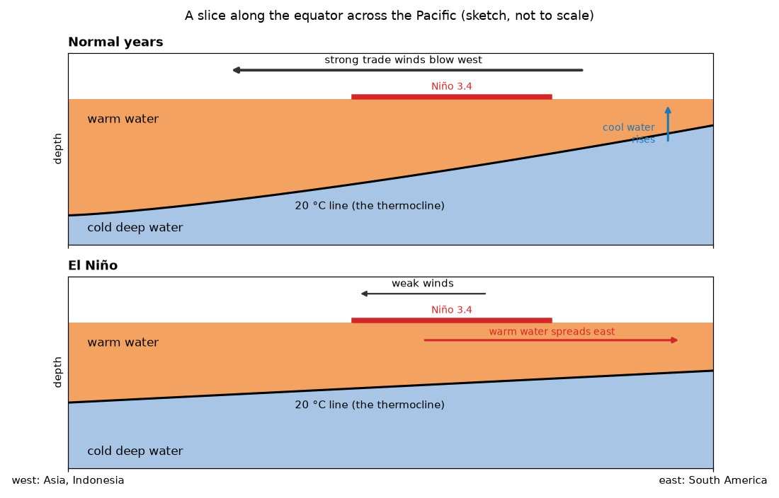
A slice along the equator, from Asia (left) to South America (right), normal years above and an El Niño below. The warm top layer ends at the 20 °C line, below which the water is cold. Normally the trade winds hold the warm water in the west and the 20 °C line comes close to the surface in the east; in an El Niño the winds weaken, the warm layer spreads east and the line flattens. A sketch drawn for this course, not to scale.

It matters far beyond the Pacific. NOAA's buoy laboratory calls ENSO the strongest year-to-year swing of climate on the planet: it shifts where rain and drought fall, and so affects farming, water and energy supplies and the lives of millions of people, as well as the Pacific's fisheries, such as tuna and anchovy. A warning a season ahead gives people time to prepare, which is why forecasting El Niño matters.

It is measured in boxes along the equator, and below the surface by buoys. The next cell draws the boxes on a map. The main one, Niño 3.4, runs from 5°S to 5°N and from 170°W to 120°W. The black triangles are the TAO array of moored buoys, as PMEL lists the sites in place by the end of 1994: each buoy measures the wind, the sea-surface temperature and the water temperature at ten depths below the surface. Section 4 uses what they measure below the surface.

In [ ]:

coast = pd.read_csv(CACHE + "/coastlines.csv")
lon = coast["lon"] % 360                                    # 0 to 360, so the Pacific is in one piece
same_line = (coast["segment"].diff() == 0) & (np.abs(lon.diff()) < 180)
lat = coast["lat"].where(same_line)                         # a blank breaks the line between segments

# the boxes NOAA's Climate Prediction Center averages: west, east, south, north (degrees east)
boxes = {"Niño 4": (160, 210, -5, 5), "Niño 3.4": (190, 240, -5, 5),
         "Niño 3": (210, 270, -5, 5), "Niño 1+2": (270, 280, -10, 0)}

plt.figure(figsize=(11, 4))
plt.plot(lon, lat, color="0.5", lw=0.6)
for name, (west, east, south, north) in boxes.items():
    colour = "tab:red" if name == "Niño 3.4" else "0.4"
    width = 2.5 if name == "Niño 3.4" else 1
    plt.plot([west, east, east, west, west], [south, south, north, north, south], color=colour, lw=width)
    plt.text((west + east) / 2, north + 1, name, color=colour, ha="center", fontsize=9)
plt.plot([120, 280, 280, 120, 120], [-5, -5, 5, 5, -5], color="tab:blue", ls=":", lw=1.5,
         label="warm water volume region (section 4)")

# the TAO moorings in place by the end of 1994, from PMEL's list of sites: latitudes at each longitude
moorings = {137: [5], 147: [0, 2, 5], 156: [-5, -2, 2, 5, 8],
            165: [-8, -5, -2, 0, 2, 5, 8], 180: [-8, -5, -2, 0, 2, 5, 8], 190: [-8, -5, -2, 0, 2, 5, 8],
            205: [-8, -5, -2, 0, 2, 5, 8], 220: [-5, -2, 0, 2, 5, 9], 235: [-8, -5, -2, 0, 2, 5, 8],
            250: [-8, -5, -2, 0, 2, 5, 8], 265: [-8, -5, -2, 0, 2, 5, 8]}
for lon_east, lats in moorings.items():
    plt.plot([lon_east] * len(lats), lats, "k^", ms=4)
plt.plot([], [], "k^", ms=4, label="TAO buoys in place by 1994")
plt.xlim(100, 300)
plt.ylim(-30, 30)
plt.gca().set_aspect("equal")
plt.xticks([120, 150, 180, 210, 240, 280], ["120°E", "150°E", "180°", "150°W", "120°W", "80°W"])
plt.xlabel("longitude")
plt.ylabel("latitude (degrees)")
plt.title("Where El Niño is measured: the Niño boxes and the TAO buoys along the equator")
plt.legend(loc="lower left", fontsize=9)
plt.show()

coast = pd.read_csv(CACHE + "/coastlines.csv") lon = coast["lon"] % 360 # 0 to 360, so the Pacific is in one piece same_line = (coast["segment"].diff() == 0) & (np.abs(lon.diff()) < 180) lat = coast["lat"].where(same_line) # a blank breaks the line between segments # the boxes NOAA's Climate Prediction Center averages: west, east, south, north (degrees east) boxes = {"Niño 4": (160, 210, -5, 5), "Niño 3.4": (190, 240, -5, 5), "Niño 3": (210, 270, -5, 5), "Niño 1+2": (270, 280, -10, 0)} plt.figure(figsize=(11, 4)) plt.plot(lon, lat, color="0.5", lw=0.6) for name, (west, east, south, north) in boxes.items(): colour = "tab:red" if name == "Niño 3.4" else "0.4" width = 2.5 if name == "Niño 3.4" else 1 plt.plot([west, east, east, west, west], [south, south, north, north, south], color=colour, lw=width) plt.text((west + east) / 2, north + 1, name, color=colour, ha="center", fontsize=9) plt.plot([120, 280, 280, 120, 120], [-5, -5, 5, 5, -5], color="tab:blue", ls=":", lw=1.5, label="warm water volume region (section 4)") # the TAO moorings in place by the end of 1994, from PMEL's list of sites: latitudes at each longitude moorings = {137: [5], 147: [0, 2, 5], 156: [-5, -2, 2, 5, 8], 165: [-8, -5, -2, 0, 2, 5, 8], 180: [-8, -5, -2, 0, 2, 5, 8], 190: [-8, -5, -2, 0, 2, 5, 8], 205: [-8, -5, -2, 0, 2, 5, 8], 220: [-5, -2, 0, 2, 5, 9], 235: [-8, -5, -2, 0, 2, 5, 8], 250: [-8, -5, -2, 0, 2, 5, 8], 265: [-8, -5, -2, 0, 2, 5, 8]} for lon_east, lats in moorings.items(): plt.plot([lon_east] * len(lats), lats, "k^", ms=4) plt.plot([], [], "k^", ms=4, label="TAO buoys in place by 1994") plt.xlim(100, 300) plt.ylim(-30, 30) plt.gca().set_aspect("equal") plt.xticks([120, 150, 180, 210, 240, 280], ["120°E", "150°E", "180°", "150°W", "120°W", "80°W"]) plt.xlabel("longitude") plt.ylabel("latitude (degrees)") plt.title("Where El Niño is measured: the Niño boxes and the TAO buoys along the equator") plt.legend(loc="lower left", fontsize=9) plt.show()

The Niño 3.4 box sits in the middle of the Pacific, between Asia and the Americas.

The data. NOAA's daily sea-surface temperature analysis (OISST) blends measurements from satellites, ships, buoys and floats onto a global grid, from September 1981 on. The Climate Prediction Center averages it over the Niño 3.4 box each month and subtracts the usual temperature for that calendar month (the 1991–2020 average). The result, nino34, is an anomaly: +1 °C in December means one degree warmer than a usual December. NOAA speaks of El Niño conditions when the anomaly stays at +0.5 °C or more, and of La Niña at −0.5 °C or less.

The next cell draws every month of the file, and marks the biggest El Niños.

In [ ]:

plt.figure(figsize=(11, 4.5))
plt.axvspan(2018, 2025 + 10 / 12, color="0.92", label="held back for the leaderboard")
plt.plot(enso["time"], enso["nino34"], color="0.25", lw=1)
plt.axhline(0.5, color="tab:red", ls="--", lw=1, label="+0.5 °C: El Niño")
plt.axhline(-0.5, color="tab:blue", ls="--", lw=1, label="-0.5 °C: La Niña")
for label, start in [("1982-83", 1982), ("1997-98", 1997), ("2015-16", 2015), ("2026", 2026)]:
    window = enso[(enso["time"] >= start + 0.5) & (enso["time"] < start + 1.5)]
    top = window.iloc[np.argmax(window["nino34"].values)]
    plt.annotate(label, (top["time"], top["nino34"]), xytext=(0, 6), textcoords="offset points",
                 ha="center", fontsize=9, color="tab:red")
plt.ylim(-3, 4)
plt.xlabel("year")
plt.ylabel("Niño 3.4 anomaly (°C)")
plt.title(f"Niño 3.4 anomaly, {(~blank).sum()} months with values, from January 1982")
plt.legend(loc="upper left", fontsize=9, ncol=3)
plt.show()

plt.figure(figsize=(11, 4.5)) plt.axvspan(2018, 2025 + 10 / 12, color="0.92", label="held back for the leaderboard") plt.plot(enso["time"], enso["nino34"], color="0.25", lw=1) plt.axhline(0.5, color="tab:red", ls="--", lw=1, label="+0.5 °C: El Niño") plt.axhline(-0.5, color="tab:blue", ls="--", lw=1, label="-0.5 °C: La Niña") for label, start in [("1982-83", 1982), ("1997-98", 1997), ("2015-16", 2015), ("2026", 2026)]: window = enso[(enso["time"] >= start + 0.5) & (enso["time"] < start + 1.5)] top = window.iloc[np.argmax(window["nino34"].values)] plt.annotate(label, (top["time"], top["nino34"]), xytext=(0, 6), textcoords="offset points", ha="center", fontsize=9, color="tab:red") plt.ylim(-3, 4) plt.xlabel("year") plt.ylabel("Niño 3.4 anomaly (°C)") plt.title(f"Niño 3.4 anomaly, {(~blank).sum()} months with values, from January 1982") plt.legend(loc="upper left", fontsize=9, ncol=3) plt.show()

The anomaly swings up and down every few years, and in 2026 the monthly anomaly climbs higher than in any El Niño before it. An El Niño builds through the northern summer and peaks around December, so its strongest month can fall in either of two calendar years. To give each El Niño one number, count a year from July to the next June: an El Niño year. July 1997 to June 1998 is El Niño year 1997.

✏️ Your turn 1¶

How does the peak of the 2026 El Niño rank among the El Niño years in the file?

Why: before forecasting anything, see what is being forecast, and how unusual this year is.

Look back at: groupby, from Earth's elevation has two peaks (03_two_peaks.ipynb).

1. Add the column el_nino_year to enso: the year for July to December, and the year minus one for January to June.
2. peak_by_year: the highest nino34 in each El Niño year. Years with no values (the held-back ones) come out blank; drop them.
3. Print the five strongest, highest first.
4. rank_2026: the place of El Niño year 2026 in that order, 1 for the strongest. Count how many years peaked higher, and add one. Print it.

Some El Niño years are only partly in the file, because the file starts in January 1982 and the held-back months are blank: 1981 (January 1982 to June 1982); 2017 (July 2017 to December 2017); 2025 (November 2025 to June 2026); 2026 (July 2026 to October 2026). Their peak is the highest of the months there are, so a partial year may rank lower than it really was. Keep them; 2026 is one of them.

Use these names, because the self-check looks for them: peak_by_year, rank_2026.

In [ ]:

# ← your answer here: write your code here
# the self-check reads: peak_by_year, rank_2026

# ← your answer here: write your code here # the self-check reads: peak_by_year, rank_2026

In [ ]:

# Self-check: run this after your answer. You do not need to read it — it only says whether something is off.
peaks = pd.Series(peak_by_year, dtype=float)
assert peaks.notna().all() and 37 <= len(peaks) <= 40, \
    "peak_by_year: one highest nino34 for each El Niño year that has values, the blank years dropped"
assert abs(peaks[1983] - (-0.16)) < 0.01, \
    "El Niño year 1983 runs from July 1983 to June 1984: January to June belong to the year before"
assert abs(peaks[2026] - 3.25) < 0.01, "the peak of El Niño year 2026 so far"
assert rank_2026 == 1 + np.sum(peaks > peaks[2026]), "rank_2026: 1 plus the number of years that peaked higher"
print(f"✓ Your turn 1 — El Niño year 2026 peaks at {peaks[2026]:+.2f} °C and ranks {rank_2026} of {len(peaks)}")

# Self-check: run this after your answer. You do not need to read it — it only says whether something is off. peaks = pd.Series(peak_by_year, dtype=float) assert peaks.notna().all() and 37 <= len(peaks) <= 40, \ "peak_by_year: one highest nino34 for each El Niño year that has values, the blank years dropped" assert abs(peaks[1983] - (-0.16)) < 0.01, \ "El Niño year 1983 runs from July 1983 to June 1984: January to June belong to the year before" assert abs(peaks[2026] - 3.25) < 0.01, "the peak of El Niño year 2026 so far" assert rank_2026 == 1 + np.sum(peaks > peaks[2026]), "rank_2026: 1 plus the number of years that peaked higher" print(f"✓ Your turn 1 — El Niño year 2026 peaks at {peaks[2026]:+.2f} °C and ranks {rank_2026} of {len(peaks)}")

In [ ]:

peaks = pd.Series(peak_by_year)   # Your turn 1, as a table whether you made a dict or a Series
colours = ["tab:red" if year == 2026 else "0.6" for year in peaks.index]
plt.figure(figsize=(11, 4))
plt.bar(peaks.index, peaks.values, color=colours)
plt.axhline(0.5, color="k", ls="--", lw=1, label="+0.5 °C: El Niño")
top_four = peaks.sort_values(ascending=False).index[:4]
for year in top_four:
    plt.text(year, peaks[year] + 0.08, f"{peaks[year]:.2f}", ha="center", fontsize=9)
plt.ylim(-1.2, 3.8)
plt.xlabel("El Niño year (July to June)")
plt.ylabel("highest Niño 3.4 anomaly (°C)")
plt.title(f"The peak of each El Niño year, {len(peaks)} years (2026 in red, so far)")
plt.legend(fontsize=9)
plt.show()

peaks = pd.Series(peak_by_year) # Your turn 1, as a table whether you made a dict or a Series colours = ["tab:red" if year == 2026 else "0.6" for year in peaks.index] plt.figure(figsize=(11, 4)) plt.bar(peaks.index, peaks.values, color=colours) plt.axhline(0.5, color="k", ls="--", lw=1, label="+0.5 °C: El Niño") top_four = peaks.sort_values(ascending=False).index[:4] for year in top_four: plt.text(year, peaks[year] + 0.08, f"{peaks[year]:.2f}", ha="center", fontsize=9) plt.ylim(-1.2, 3.8) plt.xlabel("El Niño year (July to June)") plt.ylabel("highest Niño 3.4 anomaly (°C)") plt.title(f"The peak of each El Niño year, {len(peaks)} years (2026 in red, so far)") plt.legend(fontsize=9) plt.show()

By its warmest month, 2026 is already the strongest El Niño year in the file, ahead of 2015 (+2.72 °C), 1982 and 1997, and its winter peak is probably still to come. The held-back years 2018 to 2025 had no month as warm as October 2026 either.

Why forecast it from data? Forecasting centres run two kinds of model: physical models of the ocean and air, and statistical models fitted to the past record, like the ones you will build. A study of twenty real-time forecast models found them less skilful in 2002–2011 than models had been in the 1980s and 1990s, because that decade was harder to predict (Barnston and others, 2012, doi:10.1175/BAMS-D-11-00111.1). How far ahead an El Niño can be seen, and which measurements give warning, are still open questions. Section 2 starts with the simplest forecasts.

2. How far ahead does "the same as now" work?¶

A forecast made in one month for a month later is made at a lead. In this project the leaderboard asks for a lead of 3 months: in September, the anomaly in December.

Start with two baselines, forecasts that need no model at all.

Baseline: Write the dumbest rule you can, first. Any model that cannot beat it is decoration.

• zero: the usual temperature for the month, so an anomaly of 0;
• persistence: the same anomaly as now.

Each forecast is scored by its typical miss, in °C.

Typical miss: Square every gap between what happened and what the curve said, average the squares, and take the square root: the usual size of a miss, in the data's own units.

To compare a month with the month 3 later, line the two up in one row. .shift(-3) moves a column up by three rows, so each row holds the value from three rows below. Because the file has one row for every month, three rows below is three months later. A simple case first:

In [ ]:

numbers = pd.Series([10, 20, 30, 40, 50, 60])
print(pd.DataFrame({"now": numbers, "three rows later": numbers.shift(-3)}))

numbers = pd.Series([10, 20, 30, 40, 50, 60]) print(pd.DataFrame({"now": numbers, "three rows later": numbers.shift(-3)}))

The last three rows have no value three rows later, so they come out blank (NaN). The same happens at the edges of the held-back years. Leave those rows out of any score.

✏️ Your turn 2¶

Three months ahead, how far off are "zero" and "the same as now"?

Why: these are the bars any model must clear. The leaderboard's pass line is zero.

Look back at: the typical miss, from When will CO2 pass 450 ppm? (07_co2_450_ppm.ipynb).

1. Write a function typical_miss(errors) that takes a column of errors and returns their typical miss. You will use it for every forecast in this notebook.
2. Add the column nino34_in_3 to enso: the anomaly three months after each row's month.
3. Keep the rows that have both nino34 and nino34_in_3.
4. persistence_miss: the typical miss of persistence on those rows, the anomaly three months later minus the anomaly now. zero_miss: the typical miss of forecasting 0. Print both, in °C.

Use these names, because the self-check looks for them: typical_miss, persistence_miss, zero_miss.

In [ ]:

# ← your answer here: write your code here
# the self-check reads: typical_miss, persistence_miss, zero_miss

# ← your answer here: write your code here # the self-check reads: typical_miss, persistence_miss, zero_miss

In [ ]:

# Self-check: run this after your answer. You do not need to read it — it only says whether something is off.
assert abs(typical_miss(np.array([3.0, -4.0])) - np.sqrt(12.5)) < 1e-9, \
    "the typical miss of the errors 3 and -4 is the square root of (9 + 16) / 2"
july_1997 = enso[(enso["year"] == 1997) & (enso["month"] == 7)].index[0]
assert abs(enso.loc[july_1997, "nino34_in_3"] - enso.loc[july_1997 + 3, "nino34"]) < 1e-9, \
    "nino34_in_3 in July 1997 should be the anomaly of October 1997: three months LATER, so shift up (-3)"
assert abs(persistence_miss - 0.6217) < 0.01, \
    "persistence: the anomaly three months later minus the anomaly now, on rows that have both"
assert abs(zero_miss - 0.8921) < 0.01, "zero: the typical miss of the anomaly three months later itself"
print(f"✓ Your turn 2 — three months ahead, persistence misses by {persistence_miss:.2f} °C, zero by {zero_miss:.2f} °C")

# Self-check: run this after your answer. You do not need to read it — it only says whether something is off. assert abs(typical_miss(np.array([3.0, -4.0])) - np.sqrt(12.5)) < 1e-9, \ "the typical miss of the errors 3 and -4 is the square root of (9 + 16) / 2" july_1997 = enso[(enso["year"] == 1997) & (enso["month"] == 7)].index[0] assert abs(enso.loc[july_1997, "nino34_in_3"] - enso.loc[july_1997 + 3, "nino34"]) < 1e-9, \ "nino34_in_3 in July 1997 should be the anomaly of October 1997: three months LATER, so shift up (-3)" assert abs(persistence_miss - 0.6217) < 0.01, \ "persistence: the anomaly three months later minus the anomaly now, on rows that have both" assert abs(zero_miss - 0.8921) < 0.01, "zero: the typical miss of the anomaly three months later itself" print(f"✓ Your turn 2 — three months ahead, persistence misses by {persistence_miss:.2f} °C, zero by {zero_miss:.2f} °C")

Three months ahead, "the same as now" misses by 0.62 °C and zero by 0.89 °C. Persistence wins at this lead. But an El Niño lasts about a year and then turns, so "the same as now" must get worse the further ahead it looks. How far?

✏️ Your turn 3¶

At what lead does "the same as now" become worse than forecasting zero?

Why: a forecast is only worth making where it beats the usual. This tells you how far ahead the present alone can see.

Look back at: loops that fill a dictionary and a plot of two lines, from When will CO2 pass 450 ppm? (07_co2_450_ppm.ipynb), and your Your turn 2.

1. For each lead from 1 to 12 months: the anomaly that many months later (.shift), the rows that have both values, and the typical miss of persistence and of zero on those rows.
2. persistence_by_lead and zero_by_lead: those misses, keyed by the lead (a dict or a Series). Print them. At a lead of 3 they are your persistence_miss and zero_miss.
3. first_lead_worse: the smallest lead at which persistence misses by more than zero. Print it.
4. Plot both misses (up) against the lead (across) on one figure, with a vertical line at first_lead_worse, labelled axes and a legend.

Use these names, because the self-check looks for them: persistence_by_lead, zero_by_lead, first_lead_worse.

In [ ]:

# ← your answer here: write your code here
# the self-check reads: persistence_by_lead, zero_by_lead, first_lead_worse

# ← your answer here: write your code here # the self-check reads: persistence_by_lead, zero_by_lead, first_lead_worse

In [ ]:

# Self-check: run this after your answer. You do not need to read it — it only says whether something is off.
by_lead = pd.Series(persistence_by_lead, dtype=float)
zero_lead = pd.Series(zero_by_lead, dtype=float)
assert len(by_lead) >= 12 and abs(by_lead[3] - persistence_miss) < 0.01, \
    "persistence_by_lead: the miss for each lead from 1 to 12; at a lead of 3 it is your persistence_miss"
assert by_lead[1] < by_lead[6] < by_lead[12], "persistence should miss by more the further ahead it looks"
assert abs(zero_lead[3] - zero_miss) < 0.01, "zero_by_lead: at a lead of 3 it is your zero_miss"
worse = [lead for lead in by_lead.index if by_lead[lead] > zero_lead[lead]]
assert first_lead_worse == worse[0], "first_lead_worse: the smallest lead where persistence misses by more than zero"
print(f"✓ Your turn 3 — persistence is worse than zero from a lead of {first_lead_worse} months")

# Self-check: run this after your answer. You do not need to read it — it only says whether something is off. by_lead = pd.Series(persistence_by_lead, dtype=float) zero_lead = pd.Series(zero_by_lead, dtype=float) assert len(by_lead) >= 12 and abs(by_lead[3] - persistence_miss) < 0.01, \ "persistence_by_lead: the miss for each lead from 1 to 12; at a lead of 3 it is your persistence_miss" assert by_lead[1] < by_lead[6] < by_lead[12], "persistence should miss by more the further ahead it looks" assert abs(zero_lead[3] - zero_miss) < 0.01, "zero_by_lead: at a lead of 3 it is your zero_miss" worse = [lead for lead in by_lead.index if by_lead[lead] > zero_lead[lead]] assert first_lead_worse == worse[0], "first_lead_worse: the smallest lead where persistence misses by more than zero" print(f"✓ Your turn 3 — persistence is worse than zero from a lead of {first_lead_worse} months")

From a lead of 6 months, "the same as now" is worse than forecasting the usual; a year ahead it misses by 1.23 °C against 0.89. An anomaly half a year old has often turned the other way. To see further, a forecast must know how anomalies change, and that is what a fitted line can learn.

3. Does a fitted line do better, and why does the start month matter?¶

A line can learn from the record how much of today's anomaly is left three months later. Fit nino34_in_3 on nino34 by linear regression: the slope is the share that remains, and the intercept the drift.

Linear regression: Draw the best straight line. Best means the smallest root mean squared error: the line that misses its points least.

But a line must be scored on months it did not learn from.

Train/test split: Hide some data from yourself, then check.

Split by structure: by time, not at random. Here a random split would not just be kind, it would leak the answers: the target of June is the input of September, so a model that trained on September's row has already seen June's answer. And the leaderboard hides whole years. So fit on the months up to 2009 and test on 2010 to 2017, the last years in your file before the held-back ones.

✏️ Your turn 4¶

On years it has not seen, does one fitted line beat persistence?

Why: this is the fair test every later model in this notebook is judged on.

Look back at: LinearRegression, from How old is the universe? (06_age_of_the_universe.ipynb), and the split by time, from When will CO2 pass 450 ppm? (07_co2_450_ppm.ipynb).

1. pairs: the rows of enso up to 2017 that have both nino34 and nino34_in_3.
2. fit_part: the rows of pairs up to 2009. test_part: the rows from 2010 on. Take a .copy() of each, because you will add columns. Print how many rows each holds.
3. Fit a LinearRegression of nino34_in_3 on nino34, on fit_part only. Name it line_fit, and print its slope and intercept.
4. Add its forecast for each test month as the column line of test_part.
5. line_test_miss and persistence_test_miss: the typical miss of the line and of persistence on test_part. Print both.

Use these names, because the self-check looks for them: pairs, fit_part, test_part, line_fit, line_test_miss, persistence_test_miss.

In [ ]:

# ← your answer here: write your code here
# the self-check reads: pairs, fit_part, test_part, line_fit, line_test_miss, persistence_test_miss

# ← your answer here: write your code here # the self-check reads: pairs, fit_part, test_part, line_fit, line_test_miss, persistence_test_miss

In [ ]:

# Self-check: run this after your answer. You do not need to read it — it only says whether something is off.
assert len(pairs) == 429 and pairs["year"].max() == 2017, \
    "pairs: every month up to 2017 with an anomaly now and three months later"
assert fit_part["year"].max() == 2009 and set(test_part["year"]) == set(range(2010, 2018)), \
    "split by TIME: fit_part is every pair up to 2009, test_part every pair from 2010 to 2017"
assert len(fit_part) + len(test_part) == len(pairs), "every pair is in exactly one part"
assert abs(line_test_miss - 0.6300) < 0.01, \
    "fit nino34_in_3 on nino34 using fit_part only; the typical miss of its forecast on test_part"
assert abs(persistence_test_miss - 0.6856) < 0.01, \
    "persistence on test_part: nino34_in_3 minus nino34"
print(f"✓ Your turn 4 — on 2010-2017 one line misses by {line_test_miss:.2f} °C, persistence by {persistence_test_miss:.2f} °C")

# Self-check: run this after your answer. You do not need to read it — it only says whether something is off. assert len(pairs) == 429 and pairs["year"].max() == 2017, \ "pairs: every month up to 2017 with an anomaly now and three months later" assert fit_part["year"].max() == 2009 and set(test_part["year"]) == set(range(2010, 2018)), \ "split by TIME: fit_part is every pair up to 2009, test_part every pair from 2010 to 2017" assert len(fit_part) + len(test_part) == len(pairs), "every pair is in exactly one part" assert abs(line_test_miss - 0.6300) < 0.01, \ "fit nino34_in_3 on nino34 using fit_part only; the typical miss of its forecast on test_part" assert abs(persistence_test_miss - 0.6856) < 0.01, \ "persistence on test_part: nino34_in_3 minus nino34" print(f"✓ Your turn 4 — on 2010-2017 one line misses by {line_test_miss:.2f} °C, persistence by {persistence_test_miss:.2f} °C")

One line misses the test years by 0.63 °C, persistence by 0.69 °C. The fitted slope, 0.77, says that on average about 77% of an anomaly is left three months later. But is that true in every season? An El Niño grows through one part of the year and fades through another, so the share that is left may depend on the month the forecast starts in.

✏️ Your turn 5¶

How much of an anomaly is left three months later, for each start month?

Why: if the share differs by month, one line for every month must be wrong somewhere.

Look back at: loops, masks and LinearRegression, and your Your turn 4.

1. For each start month from 1 to 12: the rows of fit_part in that month; fit a LinearRegression of nino34_in_3 on nino34 on those rows; keep its slope.
2. slope_by_month: the twelve slopes, keyed by the month (a dict or a Series). Print it.
3. weakest_month: the start month with the smallest slope. Print it.
4. Draw the slopes as bars against the month, with a dashed line at the slope of your one line, a line at 1, the spring start months (3 to 5) shaded (plt.axvspan(2.5, 5.5, ...)), labelled axes and a legend.

Use these names, because the self-check looks for them: slope_by_month, weakest_month.

In [ ]:

# ← your answer here: write your code here
# the self-check reads: slope_by_month, weakest_month

# ← your answer here: write your code here # the self-check reads: slope_by_month, weakest_month

In [ ]:

# Self-check: run this after your answer. You do not need to read it — it only says whether something is off.
slopes = pd.Series(slope_by_month, dtype=float)
assert len(slopes) == 12, "slope_by_month: one slope for each start month 1 to 12"
for month in [4, 9]:
    rows = fit_part[fit_part["month"] == month]
    slope = LinearRegression().fit(rows[["nino34"]], rows["nino34_in_3"]).coef_[0]
    assert abs(slopes[month] - slope) < 0.01, f"the slope for start month {month}: fit on the rows of fit_part in that month only"
assert weakest_month == slopes.index[np.argmin(slopes.values)], "weakest_month: the month with the smallest slope"
print(f"✓ Your turn 5 — slopes from {np.min(slopes):.2f} (month {weakest_month}) to {np.max(slopes):.2f}")

# Self-check: run this after your answer. You do not need to read it — it only says whether something is off. slopes = pd.Series(slope_by_month, dtype=float) assert len(slopes) == 12, "slope_by_month: one slope for each start month 1 to 12" for month in [4, 9]: rows = fit_part[fit_part["month"] == month] slope = LinearRegression().fit(rows[["nino34"]], rows["nino34_in_3"]).coef_[0] assert abs(slopes[month] - slope) < 0.01, f"the slope for start month {month}: fit on the rows of fit_part in that month only" assert weakest_month == slopes.index[np.argmin(slopes.values)], "weakest_month: the month with the smallest slope" print(f"✓ Your turn 5 — slopes from {np.min(slopes):.2f} (month {weakest_month}) to {np.max(slopes):.2f}")

The share left three months later depends strongly on the start month. From March only 35% of an anomaly is left by June; from July, August, September, October the slope is above 1: an anomaly in the northern summer tends to grow into the winter. One line, with 0.77 for every month, is too small in summer and too large in spring.

This is the spring predictability barrier. El Niño and La Niña are tied to the seasons: they grow from the northern summer, peak around December and fade in spring, when a new one may or may not start. A forecast that starts in spring has the least to go on. Forecasting centres see the same: a study of twenty real-time forecast models found that start times just before the middle of the year are when prediction has proven most difficult (Barnston and others, 2012, doi:10.1175/BAMS-D-11-00111.1).

✏️ Your turn 6¶

Does one line per start month forecast the test years better than one line for all?

Why: Your turn 5 says each month needs its own slope. Test it the fair way. You will reuse the function you write here for every model that follows, and for your leaderboard entry.

Look back at: functions, from How old is the universe? (06_age_of_the_universe.ipynb), and your Your turn 5.

1. Write a function per_month_forecast(fit_rows, test_rows, columns). For each start month that appears in test_rows (np.unique lists them) it fits a LinearRegression of nino34_in_3 on the given list of columns, using the rows of fit_rows in that month, and forecasts the rows of test_rows in that month. It returns the forecasts, one for each row of test_rows, in the same order.
2. Add the column per_month to test_part: your function's forecasts, fitted on fit_part with the columns ["nino34"].
3. per_month_test_miss: its typical miss. Print it beside line_test_miss.

Use these names, because the self-check looks for them: per_month_forecast, per_month_test_miss.

In [ ]:

# ← your answer here: write your code here
# the self-check reads: per_month_forecast, per_month_test_miss

# ← your answer here: write your code here # the self-check reads: per_month_forecast, per_month_test_miss

In [ ]:

# Self-check: run this after your answer. You do not need to read it — it only says whether something is off.
probe = pd.DataFrame({"month": np.repeat(np.arange(1, 13), 4), "nino34": np.tile([0.0, 1.0, 2.0, 3.0], 12)})
probe["nino34_in_3"] = probe["month"] * probe["nino34"] - 1   # month m: slope m, intercept -1
probe_test = pd.DataFrame({"month": [12, 1, 6], "nino34": [0.5, 2.0, 1.0]})
probe_out = np.asarray(per_month_forecast(probe, probe_test, ["nino34"]), dtype=float)
assert np.allclose(probe_out, [5.0, 1.0, 5.0]), \
    "per_month_forecast: for each start month that test_rows holds, fit on that month's rows of fit_rows and forecast that month's rows of test_rows, in their order"
assert abs(per_month_test_miss - 0.5336) < 0.01, \
    "fit on fit_part with the columns [\"nino34\"]; the typical miss of the forecasts on test_part"
print(f"✓ Your turn 6 — one line per month misses 2010-2017 by {per_month_test_miss:.2f} °C, one line by {line_test_miss:.2f} °C")

# Self-check: run this after your answer. You do not need to read it — it only says whether something is off. probe = pd.DataFrame({"month": np.repeat(np.arange(1, 13), 4), "nino34": np.tile([0.0, 1.0, 2.0, 3.0], 12)}) probe["nino34_in_3"] = probe["month"] * probe["nino34"] - 1 # month m: slope m, intercept -1 probe_test = pd.DataFrame({"month": [12, 1, 6], "nino34": [0.5, 2.0, 1.0]}) probe_out = np.asarray(per_month_forecast(probe, probe_test, ["nino34"]), dtype=float) assert np.allclose(probe_out, [5.0, 1.0, 5.0]), \ "per_month_forecast: for each start month that test_rows holds, fit on that month's rows of fit_rows and forecast that month's rows of test_rows, in their order" assert abs(per_month_test_miss - 0.5336) < 0.01, \ "fit on fit_part with the columns [\"nino34\"]; the typical miss of the forecasts on test_part" print(f"✓ Your turn 6 — one line per month misses 2010-2017 by {per_month_test_miss:.2f} °C, one line by {line_test_miss:.2f} °C")

Each forecast beside what came. The next cell draws, for every test month, the anomaly three months later and the two forecasts made for it.

In [ ]:

# test_part's line and per_month columns: Your turns 4 and 6
target_time = test_part["time"] + 3 / 12      # the month each forecast is FOR
plt.figure(figsize=(11, 4.5))
plt.plot(target_time, test_part["nino34_in_3"], color="k", lw=2.5, label="what came")
plt.plot(target_time, test_part["line"], "--", color="tab:orange", label=f"one line: miss {line_test_miss:.2f} °C")
plt.plot(target_time, test_part["per_month"], color="tab:purple", label=f"one line per start month: miss {per_month_test_miss:.2f} °C")
plt.axhline(0, color="0.5", lw=0.8)
plt.xlabel("year (of the month forecast)")
plt.ylabel("Niño 3.4 anomaly (°C)")
plt.title(f"Forecasts three months ahead for the {len(test_part)} test months, 2010-2017")
plt.legend(fontsize=9)
plt.show()

# test_part's line and per_month columns: Your turns 4 and 6 target_time = test_part["time"] + 3 / 12 # the month each forecast is FOR plt.figure(figsize=(11, 4.5)) plt.plot(target_time, test_part["nino34_in_3"], color="k", lw=2.5, label="what came") plt.plot(target_time, test_part["line"], "--", color="tab:orange", label=f"one line: miss {line_test_miss:.2f} °C") plt.plot(target_time, test_part["per_month"], color="tab:purple", label=f"one line per start month: miss {per_month_test_miss:.2f} °C") plt.axhline(0, color="0.5", lw=0.8) plt.xlabel("year (of the month forecast)") plt.ylabel("Niño 3.4 anomaly (°C)") plt.title(f"Forecasts three months ahead for the {len(test_part)} test months, 2010-2017") plt.legend(fontsize=9) plt.show()

One line per start month misses the test years by 0.53 °C, against 0.63 °C for one line; look at the 2015 El Niño, where one line lags behind the climb. But the test is 93 months from 8 years. Would a different 8 years agree? A bootstrap tells.

Bootstrap: Ask the data the same question a thousand times, using a different random slice of itself each time.

Here the slice is a whole year, not single months: the months of one year belong to the same El Niño or La Niña, so they miss together. And because the question is which of two models is better, use a paired bootstrap: redraw the years once, score both models on the same redraw, keep the difference, and repeat. A hard year is then hard for both, and only the difference between the models is left to vary. A redraw's typical miss is the square root of (all the squared errors its years hold ÷ all the months they hold).

✏️ Your turn 7¶

On redrawn test years, how often does one line per month beat one line?

Why: a gain is worth trusting only if it shows up year after year, not in one lucky year. You will reuse this function in section 4.

Look back at: the bootstrap, from How long was the Earth frozen? (08_how_long_frozen.ipynb).

1. Write a function paired_differences(table, new_column, old_column). Inside it:
   • add to a copy of table each row's squared error for new_column and for old_column (the error is nino34_in_3 minus the forecast);
   • one row per year: the sums of the two squared errors and the number of months;
   • make a generator, rng = np.random.default_rng(88), and an empty list. 1,000 times: redraw as many years as there are, with replacement (.sample(..., replace=True, random_state=rng)), find each model's typical miss on the redraw, and append the new miss minus the old miss;
   • return the 1,000 differences.
2. month_differences: your function on test_part, "per_month" against "line". On all the years at once the difference is per_month_test_miss minus line_test_miss.
3. month_share_better: the share of differences below zero. month_interval: their 2.5th and 97.5th percentiles. Print both.
4. Draw a histogram of the differences, with a vertical line at zero and at the two ends of the interval.

Use these names, because the self-check looks for them: paired_differences, month_differences, month_share_better, month_interval.

In [ ]:

# ← your answer here: write your code here
# the self-check reads: paired_differences, month_differences, month_share_better, month_interval

# ← your answer here: write your code here # the self-check reads: paired_differences, month_differences, month_share_better, month_interval

In [ ]:

# Self-check: run this after your answer. You do not need to read it — it only says whether something is off.
differences = np.asarray(month_differences, dtype=float)
assert len(differences) == 1000, "month_differences: one difference for each of 1,000 redraws"
assert abs(np.mean(differences) - (per_month_test_miss - line_test_miss)) < 0.03, \
    "each difference: the miss of per_month minus the miss of line, both on the same redrawn years"
assert np.std(differences) < 0.056, \
    "the differences scatter too much: score BOTH models on the same redraw, then subtract"
probe = pd.DataFrame({"year": np.repeat(np.arange(6), 12), "nino34_in_3": 0.0})
probe["old"] = 0.5
probe["new"] = np.where(probe["year"] < 3, 1.0, 0.0)
probe_spread = np.std(np.asarray(paired_differences(probe, "new", "old"), dtype=float))
assert probe_spread > 0.087, "redraw whole YEARS (one row per year), not single months"
assert abs(month_share_better - np.mean(differences < 0)) < 1e-9 and month_interval[0] < month_interval[1], \
    "month_share_better: the share of differences below zero; month_interval: the 2.5th and 97.5th percentiles"
print(f"✓ Your turn 7 — one line per month wins on {month_share_better:.0%} of redraws; difference {month_interval[0]:+.3f} to {month_interval[1]:+.3f} °C")

# Self-check: run this after your answer. You do not need to read it — it only says whether something is off. differences = np.asarray(month_differences, dtype=float) assert len(differences) == 1000, "month_differences: one difference for each of 1,000 redraws" assert abs(np.mean(differences) - (per_month_test_miss - line_test_miss)) < 0.03, \ "each difference: the miss of per_month minus the miss of line, both on the same redrawn years" assert np.std(differences) < 0.056, \ "the differences scatter too much: score BOTH models on the same redraw, then subtract" probe = pd.DataFrame({"year": np.repeat(np.arange(6), 12), "nino34_in_3": 0.0}) probe["old"] = 0.5 probe["new"] = np.where(probe["year"] < 3, 1.0, 0.0) probe_spread = np.std(np.asarray(paired_differences(probe, "new", "old"), dtype=float)) assert probe_spread > 0.087, "redraw whole YEARS (one row per year), not single months" assert abs(month_share_better - np.mean(differences < 0)) < 1e-9 and month_interval[0] < month_interval[1], \ "month_share_better: the share of differences below zero; month_interval: the 2.5th and 97.5th percentiles" print(f"✓ Your turn 7 — one line per month wins on {month_share_better:.0%} of redraws; difference {month_interval[0]:+.3f} to {month_interval[1]:+.3f} °C")

One line per month wins on 98.6% of the redrawn sets of years, and the 95% interval of the difference, -0.169 to -0.013 °C, is below zero. The start month matters, and a model that knows it forecasts better.

4. Does the ocean's stored heat help, and in every decade?¶

El Niño's fuel is stored below the surface. The tropical sea is warm only in a top layer; below it the temperature drops sharply, at the 20 °C line of the slice in section 1. The warm water volume (wwv) is the volume of that warm layer, the water warmer than 20 °C, between 5°S and 5°N across the Pacific, from 120°E to 80°W (the dotted box on the map in section 1), as an anomaly from the usual, in units of 10¹⁴ m³. NOAA's Pacific Marine Environmental Laboratory computes it every month from temperatures measured below the surface; along the equator many come from the TAO buoys (the triangles on the map), built from 1985 to 1994 to understand and predict El Niño.

What earlier research found. Using measurements from 1980–1999, years in which the buoy array was still being built, Meinen and McPhaden (2000, Journal of Climate, doi:10.1175/1520-0442(2000)013<3551:OOWWVC>2.0.CO;2) confirmed that the El Niño cycle recharges and discharges warm water along the equator: warm water piles up before an El Niño, and the El Niño drains it. They also found that larger swings in the warm water volume go with larger swings in surface temperature.

The next cell draws both records together.

In [ ]:

plt.figure(figsize=(11, 4.5))
plt.axvspan(2018, 2025 + 10 / 12, color="0.92", label="held back for the leaderboard")
plt.plot(enso["time"], enso["nino34"], color="tab:red", lw=1.2, label="Niño 3.4 anomaly (°C)")
plt.plot(enso["time"], enso["wwv"], color="tab:blue", lw=1.2, label="warm water volume anomaly (10¹⁴ m³)")
plt.axhline(0, color="k", lw=0.8)
plt.xlabel("year")
plt.ylabel("anomaly: Niño 3.4 in °C (red),\nwarm water volume in 10¹⁴ m³ (blue)")
plt.title("The Pacific's surface (red) and the heat stored below it (blue), every month of the file")
plt.legend(loc="upper left", fontsize=9, ncol=3)
plt.show()

plt.figure(figsize=(11, 4.5)) plt.axvspan(2018, 2025 + 10 / 12, color="0.92", label="held back for the leaderboard") plt.plot(enso["time"], enso["nino34"], color="tab:red", lw=1.2, label="Niño 3.4 anomaly (°C)") plt.plot(enso["time"], enso["wwv"], color="tab:blue", lw=1.2, label="warm water volume anomaly (10¹⁴ m³)") plt.axhline(0, color="k", lw=0.8) plt.xlabel("year") plt.ylabel("anomaly: Niño 3.4 in °C (red),\nwarm water volume in 10¹⁴ m³ (blue)") plt.title("The Pacific's surface (red) and the heat stored below it (blue), every month of the file") plt.legend(loc="upper left", fontsize=9, ncol=3) plt.show()

Before each big El Niño the blue line rises first, then falls as the red line peaks. How many months ahead does it run? The next cell correlates the warm water volume of each month with the Niño 3.4 anomaly some months later, up to 2017.

In [ ]:

up_to_2017 = enso[enso["year"] <= 2017]
correlation_by_lag = {}
for lag in range(0, 13):
    later = up_to_2017["nino34"].shift(-lag)
    correlation_by_lag[lag] = np.corrcoef(up_to_2017["wwv"][later.notna()], later[later.notna()])[0, 1]
correlation_by_lag = pd.Series(correlation_by_lag)
best_lag = correlation_by_lag.index[np.argmax(correlation_by_lag.values)]

plt.figure(figsize=(8, 4))
plt.bar(correlation_by_lag.index, correlation_by_lag.values, color="tab:blue")
plt.bar(best_lag, correlation_by_lag[best_lag], color="navy", label=f"strongest: {best_lag} months later")
plt.xticks(range(0, 13))
plt.xlabel("months between the warm water volume and the Niño 3.4 anomaly")
plt.ylabel("correlation")
plt.title(f"The stored heat runs ahead of the surface, {len(up_to_2017)} months to 2017")
plt.legend(fontsize=9)
plt.show()

up_to_2017 = enso[enso["year"] <= 2017] correlation_by_lag = {} for lag in range(0, 13): later = up_to_2017["nino34"].shift(-lag) correlation_by_lag[lag] = np.corrcoef(up_to_2017["wwv"][later.notna()], later[later.notna()])[0, 1] correlation_by_lag = pd.Series(correlation_by_lag) best_lag = correlation_by_lag.index[np.argmax(correlation_by_lag.values)] plt.figure(figsize=(8, 4)) plt.bar(correlation_by_lag.index, correlation_by_lag.values, color="tab:blue") plt.bar(best_lag, correlation_by_lag[best_lag], color="navy", label=f"strongest: {best_lag} months later") plt.xticks(range(0, 13)) plt.xlabel("months between the warm water volume and the Niño 3.4 anomaly") plt.ylabel("correlation") plt.title(f"The stored heat runs ahead of the surface, {len(up_to_2017)} months to 2017") plt.legend(fontsize=9) plt.show()

The warm water volume goes with the Niño 3.4 anomaly 5 months later (correlation 0.53) much more than with the same month (0.17). Three months later, the leaderboard's lead, it is 0.49. In September 2026 it stood at +3.16, higher than any month up to 2017 (largest +3.12). If it adds information that the anomaly now does not hold, a forecast with both should beat a forecast with the anomaly alone.

✏️ Your turn 8¶

Does adding the warm water volume improve the per-month forecast of the test years?

Why: this is new information about the ocean, not a new shape of model: the same lines, one more column. Test it the same fair way.

Look back at: your Your turns 6 and 7.

1. Add the column per_month_wwv to test_part: your per_month_forecast, fitted on fit_part with the columns ["nino34", "wwv"].
2. wwv_test_miss: its typical miss. Print it beside per_month_test_miss.
3. wwv_differences: your paired_differences on test_part, "per_month_wwv" against "per_month". wwv_share_better: the share below zero. wwv_interval: the 2.5th and 97.5th percentiles. Print both.

Use these names, because the self-check looks for them: wwv_test_miss, wwv_differences, wwv_share_better, wwv_interval.

In [ ]:

# ← your answer here: write your code here
# the self-check reads: wwv_test_miss, wwv_differences, wwv_share_better, wwv_interval

# ← your answer here: write your code here # the self-check reads: wwv_test_miss, wwv_differences, wwv_share_better, wwv_interval

In [ ]:

# Self-check: run this after your answer. You do not need to read it — it only says whether something is off.
assert abs(wwv_test_miss - 0.4951) < 0.01, \
    "per_month_forecast fitted on fit_part with the columns [\"nino34\", \"wwv\"]; its typical miss on test_part"
differences = np.asarray(wwv_differences, dtype=float)
assert len(differences) == 1000 and abs(np.mean(differences) - (wwv_test_miss - per_month_test_miss)) < 0.03, \
    "wwv_differences: paired_differences(test_part, \"per_month_wwv\", \"per_month\")"
assert abs(wwv_share_better - np.mean(differences < 0)) < 1e-9 and wwv_interval[0] < wwv_interval[1], \
    "wwv_share_better: the share of differences below zero; wwv_interval: the 2.5th and 97.5th percentiles"
assert 0.6 < wwv_share_better < 0.99, "with the same paired function as Your turn 7, the share should be well above a half"
print(f"✓ Your turn 8 — with wwv {wwv_test_miss:.3f} °C, without {per_month_test_miss:.3f} °C; wins on {wwv_share_better:.0%} of redraws")

# Self-check: run this after your answer. You do not need to read it — it only says whether something is off. assert abs(wwv_test_miss - 0.4951) < 0.01, \ "per_month_forecast fitted on fit_part with the columns [\"nino34\", \"wwv\"]; its typical miss on test_part" differences = np.asarray(wwv_differences, dtype=float) assert len(differences) == 1000 and abs(np.mean(differences) - (wwv_test_miss - per_month_test_miss)) < 0.03, \ "wwv_differences: paired_differences(test_part, \"per_month_wwv\", \"per_month\")" assert abs(wwv_share_better - np.mean(differences < 0)) < 1e-9 and wwv_interval[0] < wwv_interval[1], \ "wwv_share_better: the share of differences below zero; wwv_interval: the 2.5th and 97.5th percentiles" assert 0.6 < wwv_share_better < 0.99, "with the same paired function as Your turn 7, the share should be well above a half" print(f"✓ Your turn 8 — with wwv {wwv_test_miss:.3f} °C, without {per_month_test_miss:.3f} °C; wins on {wwv_share_better:.0%} of redraws")

With the warm water volume the forecast misses the test years by 0.50 °C, against 0.53 °C without it, and wins on 89% of the paired redraws. That is a real hint, but not proof: the 95% interval, -0.099 to +0.021 °C, reaches past zero. Eight years hold only a few El Niños.

A second fair test is another decade. Fit only on the years up to 1999 and test on 2000 to 2009, the decade before. If the stored heat always helps, it should help there too.

✏️ Your turn 9¶

Fitted up to 1999, does the warm water volume help forecast 2000 to 2009?

Why: an improvement found on one stretch of years should be checked on another before you bet on it.

Look back at: your Your turns 4, 6 and 8.

1. early_fit: the rows of pairs up to 1999. decade_2000s: the rows from 2000 to 2009 (a .copy()).
2. Add two columns to decade_2000s: per_month and per_month_wwv, your per_month_forecast fitted on early_fit with ["nino34"] and with ["nino34", "wwv"].
3. miss_2000s_per_month and miss_2000s_wwv: their typical misses. Print both.
4. share_2000s: with your paired_differences, the share of redraws on which the forecast with wwv wins. Print it.

Use these names, because the self-check looks for them: early_fit, decade_2000s, miss_2000s_per_month, miss_2000s_wwv, share_2000s.

In [ ]:

# ← your answer here: write your code here
# the self-check reads: early_fit, decade_2000s, miss_2000s_per_month, miss_2000s_wwv, share_2000s

# ← your answer here: write your code here # the self-check reads: early_fit, decade_2000s, miss_2000s_per_month, miss_2000s_wwv, share_2000s

In [ ]:

# Self-check: run this after your answer. You do not need to read it — it only says whether something is off.
assert early_fit["year"].max() == 1999 and set(decade_2000s["year"]) == set(range(2000, 2010)), \
    "early_fit: pairs up to 1999; decade_2000s: pairs from 2000 to 2009"
assert abs(miss_2000s_per_month - 0.3914) < 0.01, \
    "per_month_forecast fitted on early_fit with [\"nino34\"]; its typical miss on decade_2000s"
assert abs(miss_2000s_wwv - 0.3887) < 0.01, \
    "per_month_forecast fitted on early_fit with [\"nino34\", \"wwv\"]; its typical miss on decade_2000s"
assert 0.2 < share_2000s < 0.85, "share_2000s: the share of paired redraws of the 2000s on which the forecast with wwv wins"
print(f"✓ Your turn 9 — 2000-2009: with wwv {miss_2000s_wwv:.3f} °C, without {miss_2000s_per_month:.3f} °C; wins on {share_2000s:.0%} of redraws")

# Self-check: run this after your answer. You do not need to read it — it only says whether something is off. assert early_fit["year"].max() == 1999 and set(decade_2000s["year"]) == set(range(2000, 2010)), \ "early_fit: pairs up to 1999; decade_2000s: pairs from 2000 to 2009" assert abs(miss_2000s_per_month - 0.3914) < 0.01, \ "per_month_forecast fitted on early_fit with [\"nino34\"]; its typical miss on decade_2000s" assert abs(miss_2000s_wwv - 0.3887) < 0.01, \ "per_month_forecast fitted on early_fit with [\"nino34\", \"wwv\"]; its typical miss on decade_2000s" assert 0.2 < share_2000s < 0.85, "share_2000s: the share of paired redraws of the 2000s on which the forecast with wwv wins" print(f"✓ Your turn 9 — 2000-2009: with wwv {miss_2000s_wwv:.3f} °C, without {miss_2000s_per_month:.3f} °C; wins on {share_2000s:.0%} of redraws")

In the 2000s the warm water volume did not help: 0.389 °C with it, 0.391 °C without, and it wins on only 54% of the redraws, about a coin toss. You are not the first to see this. A study of the measurements from 1980 to 2010 found that in the 1980s and 1990s the warm water volume ran two to three seasons ahead of El Niño, but in 2000 to 2010 only one season, and linked the change to more El Niños centred in the middle of the Pacific rather than the east (McPhaden, 2012, doi:10.1029/2012GL051826).

So the stored heat helps in some decades and not in others. The leaderboard's years, 2018 to 2025, are a new stretch, and nobody yet knows which kind it was. That is the bet your entry makes. The next cell puts every forecast of this notebook on one chart.

In [ ]:

# the misses of Your turns 2 to 9, on the two fair tests
zero_test_miss = typical_miss(test_part["nino34_in_3"])
zero_2000s = typical_miss(decade_2000s["nino34_in_3"])
persistence_2000s = typical_miss(decade_2000s["nino34_in_3"] - decade_2000s["nino34"])
early_line = LinearRegression().fit(early_fit[["nino34"]], early_fit["nino34_in_3"])
line_2000s = typical_miss(decade_2000s["nino34_in_3"] - early_line.predict(decade_2000s[["nino34"]]))
names =["zero", "persistence", "one line", "one line\nper month", "per month\n+ wwv"]
misses_2010s = [zero_test_miss, persistence_test_miss, line_test_miss, per_month_test_miss, wwv_test_miss]
misses_2000s = [zero_2000s, persistence_2000s, line_2000s, miss_2000s_per_month, miss_2000s_wwv]
positions = np.arange(len(names))

plt.figure(figsize=(9, 4.5))
plt.bar(positions - 0.2, misses_2010s, width=0.4, color="tab:purple", label="fit to 2009, test 2010-2017")
plt.bar(positions + 0.2, misses_2000s, width=0.4, color="0.6", label="fit to 1999, test 2000-2009")
for k in range(len(names)):
    plt.text(positions[k] - 0.2, misses_2010s[k] + 0.01, f"{misses_2010s[k]:.2f}", ha="center", fontsize=8)
    plt.text(positions[k] + 0.2, misses_2000s[k] + 0.01, f"{misses_2000s[k]:.2f}", ha="center", fontsize=8)
plt.xticks(positions, names)
plt.xlabel("forecast")
plt.ylabel("typical miss three months ahead (°C)")
plt.title("Every forecast on the two fair tests (lower is better)")
plt.legend(fontsize=9)
plt.show()

# the misses of Your turns 2 to 9, on the two fair tests zero_test_miss = typical_miss(test_part["nino34_in_3"]) zero_2000s = typical_miss(decade_2000s["nino34_in_3"]) persistence_2000s = typical_miss(decade_2000s["nino34_in_3"] - decade_2000s["nino34"]) early_line = LinearRegression().fit(early_fit[["nino34"]], early_fit["nino34_in_3"]) line_2000s = typical_miss(decade_2000s["nino34_in_3"] - early_line.predict(decade_2000s[["nino34"]])) names =["zero", "persistence", "one line", "one line\nper month", "per month\n+ wwv"] misses_2010s = [zero_test_miss, persistence_test_miss, line_test_miss, per_month_test_miss, wwv_test_miss] misses_2000s = [zero_2000s, persistence_2000s, line_2000s, miss_2000s_per_month, miss_2000s_wwv] positions = np.arange(len(names)) plt.figure(figsize=(9, 4.5)) plt.bar(positions - 0.2, misses_2010s, width=0.4, color="tab:purple", label="fit to 2009, test 2010-2017") plt.bar(positions + 0.2, misses_2000s, width=0.4, color="0.6", label="fit to 1999, test 2000-2009") for k in range(len(names)): plt.text(positions[k] - 0.2, misses_2010s[k] + 0.01, f"{misses_2010s[k]:.2f}", ha="center", fontsize=8) plt.text(positions[k] + 0.2, misses_2000s[k] + 0.01, f"{misses_2000s[k]:.2f}", ha="center", fontsize=8) plt.xticks(positions, names) plt.xlabel("forecast") plt.ylabel("typical miss three months ahead (°C)") plt.title("Every forecast on the two fair tests (lower is better)") plt.legend(fontsize=9) plt.show()

The leaderboard¶

The leaderboard cannot give you a file of 2018 to 2025 inputs: each month's target is another month's input, so the file would hold the answers. Instead, your entry is a forecast table. template has one row for each start month (1 to 12), each nino34 from -2.5 to +3.5 °C in steps of 0.5, and each wwv from -5.0 to +4.0 in steps of 0.5: 2,964 rows, with an empty forecast column. You fill in the anomaly three months later that your model forecasts for each row.

• How it is read. For each of the 91 hidden start months, January 2018 to July 2025, the board takes your table's rows for that start month and reads it at that month's nino34 and wwv, along straight lines between the grid's values (a value beyond the grid is read at its edge). For a per-month line the reading is exactly your line's forecast.
• The board shows a public score, the typical miss in °C on three of the eight years. The final score, on the other five, is shown after the board closes, and your rank on it is graded.
• So choose your entry by your own fair tests, not by the public score. Three years are a few El Niños at most.
• Do not look up or download the hidden answers, the published Niño 3.4 and warm water volume values for 2018 to 2025: a table built from them is not your model, and it scores 0.

How the board reads between rows: a worked example. Say your table holds, for start month 9 and a wwv on the grid, a forecast of 1.0 °C in the row with nino34 = 2.0 and 1.4 °C in the row with nino34 = 2.5. A September with nino34 = 2.2 is read on the straight line between those two rows. The next cell does the arithmetic.

In [ ]:

# one start month, wwv on a grid value, and two neighbouring nino34 rows of a table (°C)
nino34_low, nino34_high = 2.0, 2.5           # two neighbouring nino34 values on the grid
forecast_low, forecast_high = 1.0, 1.4       # what the table holds in those two rows
nino34_month = 2.2                           # the month the board reads

share_of_the_way = (nino34_month - nino34_low) / (nino34_high - nino34_low)
value_read = forecast_low + share_of_the_way * (forecast_high - forecast_low)
print("2.2 is", round(100 * share_of_the_way), "% of the way from 2.0 to 2.5, so the board reads", round(value_read, 2), "°C")

# one start month, wwv on a grid value, and two neighbouring nino34 rows of a table (°C) nino34_low, nino34_high = 2.0, 2.5 # two neighbouring nino34 values on the grid forecast_low, forecast_high = 1.0, 1.4 # what the table holds in those two rows nino34_month = 2.2 # the month the board reads share_of_the_way = (nino34_month - nino34_low) / (nino34_high - nino34_low) value_read = forecast_low + share_of_the_way * (forecast_high - forecast_low) print("2.2 is", round(100 * share_of_the_way), "% of the way from 2.0 to 2.5, so the board reads", round(value_read, 2), "°C")

The board reads 40% of the way from 1.0 to 1.4: 1.16 °C. When wwv also falls between two grid values, it does this twice: first along wwv, then along nino34. You do not do this yourself. Fill every row with your model's forecast for that row's inputs, and the board reads the table at each hidden month.

✏️ Your turn 10¶

Your leaderboard entry: the forecast table.

Why: this is the project's answer, scored on months you have not seen, and ranked against the other students. Choose by your fair tests; the public score is three years, and your rank is decided on the other five.

Look back at: your Your turns 6, 8 and 9.

1. Take the model your tests chose: one line per start month on nino34 and wwv, unless your own tests found something better.
2. Fit it on every row of pairs, 1982 to 2017: the test years are data too, and the newest. Your per_month_forecast does this if you give it pairs to fit on and template to forecast: template has the columns month, nino34 and wwv, like pairs.
3. submission: a copy of template, with its forecast column filled with your forecasts. Save it with submission.to_csv("submission.csv", index=False).
4. Print its first rows, its number of rows and of blanks, and its lowest and highest forecast.
5. Run the self-check, then download submission.csv and this notebook and upload both together (the steps are under "What you hand in" above) to Final project: El Niño.

Use these names, because the self-check looks for them: submission.

In [ ]:

# ← your answer here: write your code here
# the self-check reads: submission

# ← your answer here: write your code here # the self-check reads: submission

In [ ]:

# Self-check: run this after your answer. You do not need to read it — it only says whether something is off.
saved = pd.read_csv("submission.csv")
assert list(saved.columns) == ["month", "nino34", "wwv", "forecast"], "submission.csv holds the template's four columns"
assert len(saved) == len(template) and np.allclose(saved[["month", "nino34", "wwv"]], template[["month", "nino34", "wwv"]]), \
    "one row per row of the template, in its order: fill the forecast column, do not change the grid"
assert saved["forecast"].notna().all(), "a forecast for every row of the template"
assert np.allclose(saved["forecast"], submission["forecast"]), "submission.csv holds the table submission"
assert np.max(np.abs(saved["forecast"])) < 10, "the forecast is the ANOMALY in °C, not the temperature"
# read the table at every month of pairs, as the leaderboard reads it at the hidden months
nino34_grid = np.sort(saved["nino34"].unique())
wwv_grid = np.sort(saved["wwv"].unique())
read = np.zeros(len(pairs))
for k, (month, nino34, wwv) in enumerate(pairs[["month", "nino34", "wwv"]].values):
    grid = saved[saved["month"] == month].pivot(index="nino34", columns="wwv", values="forecast")
    along_wwv = [np.interp(wwv, wwv_grid, grid.loc[n].values) for n in nino34_grid]
    read[k] = np.interp(nino34, nino34_grid, along_wwv)
table_miss = typical_miss(pairs["nino34_in_3"] - read)
same_as_now = typical_miss(pairs["nino34_in_3"] - pairs["nino34"])
assert table_miss < same_as_now - 0.05, \
    "read at the months of pairs, your table should beat persistence clearly: fill it with your MODEL's forecasts"
print(f"✓ Your turn 10 — submission.csv: {len(saved)} forecasts; read at the months of 1982-2017 it misses by {table_miss:.2f} °C, persistence by {same_as_now:.2f} °C")

# Self-check: run this after your answer. You do not need to read it — it only says whether something is off. saved = pd.read_csv("submission.csv") assert list(saved.columns) == ["month", "nino34", "wwv", "forecast"], "submission.csv holds the template's four columns" assert len(saved) == len(template) and np.allclose(saved[["month", "nino34", "wwv"]], template[["month", "nino34", "wwv"]]), \ "one row per row of the template, in its order: fill the forecast column, do not change the grid" assert saved["forecast"].notna().all(), "a forecast for every row of the template" assert np.allclose(saved["forecast"], submission["forecast"]), "submission.csv holds the table submission" assert np.max(np.abs(saved["forecast"])) < 10, "the forecast is the ANOMALY in °C, not the temperature" # read the table at every month of pairs, as the leaderboard reads it at the hidden months nino34_grid = np.sort(saved["nino34"].unique()) wwv_grid = np.sort(saved["wwv"].unique()) read = np.zeros(len(pairs)) for k, (month, nino34, wwv) in enumerate(pairs[["month", "nino34", "wwv"]].values): grid = saved[saved["month"] == month].pivot(index="nino34", columns="wwv", values="forecast") along_wwv = [np.interp(wwv, wwv_grid, grid.loc[n].values) for n in nino34_grid] read[k] = np.interp(nino34, nino34_grid, along_wwv) table_miss = typical_miss(pairs["nino34_in_3"] - read) same_as_now = typical_miss(pairs["nino34_in_3"] - pairs["nino34"]) assert table_miss < same_as_now - 0.05, \ "read at the months of pairs, your table should beat persistence clearly: fill it with your MODEL's forecasts" print(f"✓ Your turn 10 — submission.csv: {len(saved)} forecasts; read at the months of 1982-2017 it misses by {table_miss:.2f} °C, persistence by {same_as_now:.2f} °C")

Your table is a surface: one forecast for every pair of inputs, a different surface for each start month. The next cell draws your table for September as colours, with the Septembers of 2010 to 2017, your test years, as dots. The colour under a dot is the forecast the table gives that month, read the way the board reads a hidden month.

In [ ]:

# your table for start month 9 (Your turn 10), with the Septembers of 2010-2017 on it
september = submission[submission["month"] == 9]
table_9 = september.pivot(index="wwv", columns="nino34", values="forecast")
limit = np.max(np.abs(table_9.values))
septembers = pairs[(pairs["month"] == 9) & (pairs["year"] >= 2010)]

plt.figure(figsize=(9, 5.5))
plt.pcolormesh(table_9.columns, table_9.index, table_9.values, cmap="RdBu_r", vmin=-limit, vmax=limit, shading="nearest")
plt.colorbar(label="your forecast for December (°C)")
plt.scatter(septembers["nino34"], septembers["wwv"], color="k", s=30)
for year, nino34, wwv in septembers[["year", "nino34", "wwv"]].values:
    plt.annotate(str(int(year)), (nino34, wwv), xytext=(4, 4), textcoords="offset points", fontsize=8)
plt.xlabel("nino34 in September (°C)")
plt.ylabel("wwv in September (10¹⁴ m³)")
plt.title(f"Your table for start month 9: {len(september)} rows; dots: {len(septembers)} Septembers, 2010-2017")
plt.show()

# your table for start month 9 (Your turn 10), with the Septembers of 2010-2017 on it september = submission[submission["month"] == 9] table_9 = september.pivot(index="wwv", columns="nino34", values="forecast") limit = np.max(np.abs(table_9.values)) septembers = pairs[(pairs["month"] == 9) & (pairs["year"] >= 2010)] plt.figure(figsize=(9, 5.5)) plt.pcolormesh(table_9.columns, table_9.index, table_9.values, cmap="RdBu_r", vmin=-limit, vmax=limit, shading="nearest") plt.colorbar(label="your forecast for December (°C)") plt.scatter(septembers["nino34"], septembers["wwv"], color="k", s=30) for year, nino34, wwv in septembers[["year", "nino34", "wwv"]].values: plt.annotate(str(int(year)), (nino34, wwv), xytext=(4, 4), textcoords="offset points", fontsize=8) plt.xlabel("nino34 in September (°C)") plt.ylabel("wwv in September (10¹⁴ m³)") plt.title(f"Your table for start month 9: {len(september)} rows; dots: {len(septembers)} Septembers, 2010-2017") plt.show()

Where the colours change fastest, the inputs matter most. With one line per start month the colours change along straight bands: a warmer September, or more stored heat, means a warmer December. Every hidden month is read from a surface like this one.

In [ ]:

# the latest month with both inputs, forecast by one line per start month with wwv (Your turns 6 and 10)
latest = enso[(enso["year"] == 2026) & (enso["month"] == 9)]
forecast_dec = np.asarray(per_month_forecast(pairs, latest, ["nino34", "wwv"]))[0]
print("September 2026: nino34", latest["nino34"].values[0], " wwv", latest["wwv"].values[0])
print("your model's forecast for December 2026:", round(forecast_dec, 2), "°C")
print("the warmest month up to 2017:", np.max(pairs["nino34"]), "°C")

# the latest month with both inputs, forecast by one line per start month with wwv (Your turns 6 and 10) latest = enso[(enso["year"] == 2026) & (enso["month"] == 9)] forecast_dec = np.asarray(per_month_forecast(pairs, latest, ["nino34", "wwv"]))[0] print("September 2026: nino34", latest["nino34"].values[0], " wwv", latest["wwv"].values[0]) print("your model's forecast for December 2026:", round(forecast_dec, 2), "°C") print("the warmest month up to 2017:", np.max(pairs["nino34"]), "°C")

The question, answered¶

October 2026 was the warmest month in the Niño 3.4 record since 1982, and three months ahead it could be forecast better than "the same as now" by a model that knows the season and the ocean's stored heat. On 2010 to 2017 one line per start month cut the typical miss from 0.63 to 0.53 °C, because an anomaly grows from summer and fades through spring; the warm water volume cut it to 0.50 °C, but it did not help in the 2000s.

The open question¶

What does your model forecast for this winter's peak, and how far should you trust a line pushed past every El Niño it has seen?

Your model forecasts +3.9 °C for December 2026. Both of its inputs in September are beyond anything it was fitted on (the warmest month up to 2017 was +2.72 °C), so a straight line is carrying it into a region with no data. NOAA's Climate Prediction Center publishes its own forecasts every month, and January 2027 will bring the measurement. Compare the three. After the board closes, its final scores also show whose models held up on 2018 to 2025.