How hard will the ground shake at distance R from a magnitude M earthquake?
EPS 88 · PyEarth · final project. Open your own copy on DataHub: click here.
On 6 February 2023 two earthquakes, magnitude 7.7 and 7.5, struck southern Türkiye nine hours apart. How hard did the ground shake at each station that recorded them? In this project you build a model from earthquake recordings before 2023, most of them in Europe and the Middle East, and use it to predict the shaking in 2,327 recordings made since, those two earthquakes included. You never see the answers. The leaderboard does, and it ranks everyone's entries.
This notebook is built like a weekly notebook: a few questions lead it, each section answers one, and every place you work opens with a pencil icon ✏️ and the words Your turn. The difference is how much you write. Each Your turn says why the step matters and gives a numbered plan in words; the cell under it is empty, and you write all of the code, looking back at the weekly notebook it names. A self-check cell follows. Run it: it tells you whether your numbers are right, as in every week.
The last Your turn is your leaderboard entry: it saves the file submission.csv. Run every cell so your answers and figures are saved in the file, then download this notebook itself — the .ipynb file — and upload it to Gradescope together with submission.csv. In JupyterLab: File ▸ Download, or right-click the file in the left-hand panel and choose Download. The leaderboard scores your file on answers you never see and ranks everyone's entries.
Two habits from the first minute. A cell runs when you press Shift+Enter, and the notebook remembers everything it has already run — so when something breaks and you cannot see why, Kernel → Restart Kernel and Run All Cells throws the memory away and rebuilds it from the top. That is never the wrong thing to do.
Background
On 6 February 2023, the ground under southern Türkiye shook hard enough to bring down a hospital. (The two earthquakes are magnitude 7.7 and 7.5 in this project's data; the US Geological Survey gives 7.8 and 7.5.) In the photo, from Antakya, one wing of the Hatay hospital has collapsed and the wing beside it still stands. Whether a building stands depends on how hard the ground under it shakes, and on whether it was built for that shaking.
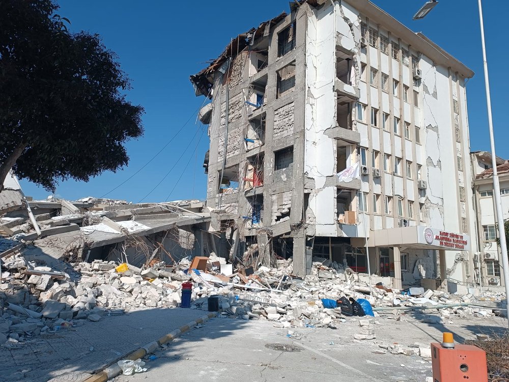
Hatay Training and Research Hospital, Antakya, after the earthquakes. Photo: Mustafa Kuzugüdemn (CC0), via Wikimedia Commons.

The cost was enormous, and the danger was already on the map. More than 53,000 people died in Türkiye and more than 5,900 in Syria. An inspection found 164,000 buildings destroyed or badly damaged, and the damage in Türkiye was put at US$150 billion, about 9% of its economy (all from Wikipedia, 2023 Turkey–Syria earthquakes). A seismic hazard map like the one below shows how hard the ground is likely to shake at each place: here, the peak ground acceleration that has a 10% chance of being passed in 50 years. The south-east of Türkiye, where the plate boundary (black line) runs north from Syria into Türkiye, is coloured for strong shaking. Engineers design buildings for the shaking such maps give.
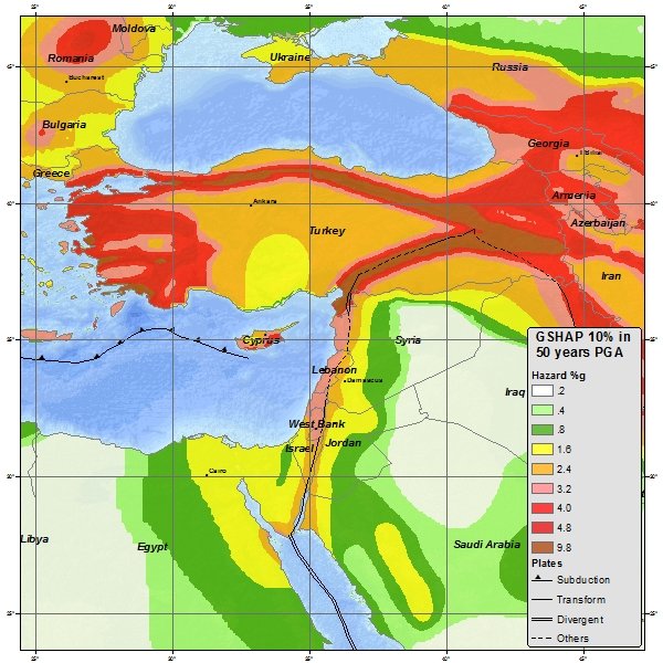
Seismic hazard of Türkiye and its neighbours, from the Global Seismic Hazard Assessment Program. The legend says "%g", but its numbers, 0.2 to 9.8, are in m/s², the unit of the GSHAP data: 9.8 m/s² is 1 g, so 4.8 m/s² is about half of g. Map: USGS (public domain), via Wikimedia Commons.

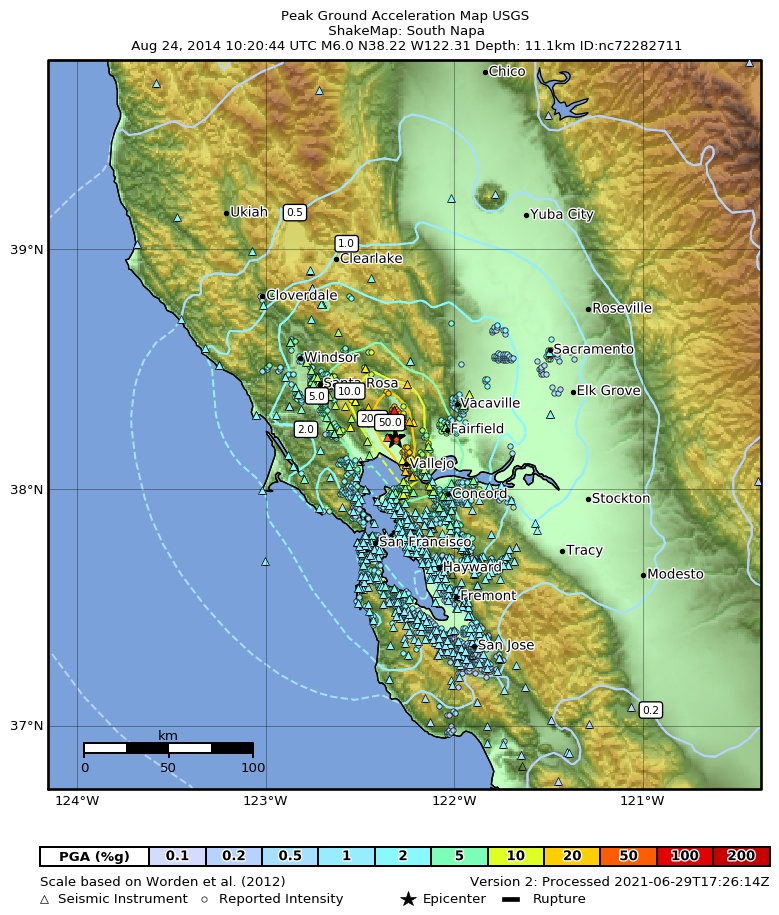
Every hazard map and every shaking map rests on a ground-motion model. Stations are few, so nobody measures the shaking at every building. A ground-motion model fills the gaps: from an earthquake's magnitude, the distance to a site and the ground under it, it predicts how hard that site shakes. A hazard map runs it for every earthquake that could happen; after a real one, a shaking map uses it between the stations. California has the same problem. The USGS ShakeMap below, for the magnitude 6.0 South Napa earthquake of 2014, colours the peak acceleration everywhere, though its stations (triangles) sit only in some places. Building a model that predicts well at a place it has never measured is the job of this project.
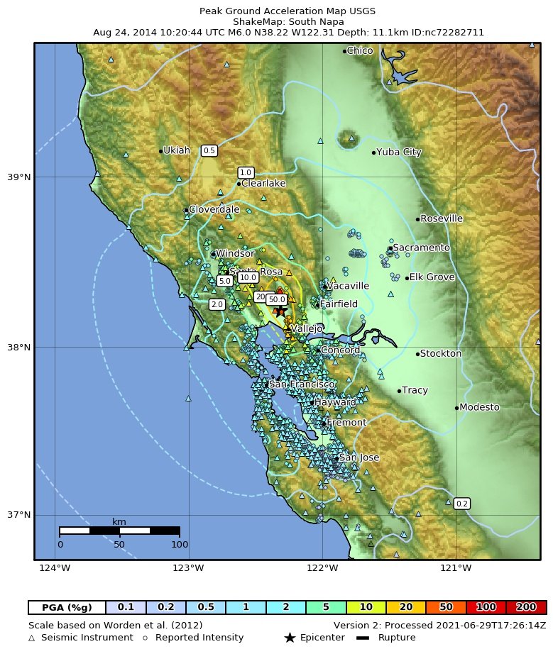
Peak ground acceleration (% of g) in the 2014 South Napa earthquake. USGS ShakeMap (public domain).
Your data: 34,481 recordings from the Engineering Strong Motion database (ESM). Each one was made by an accelerometer like the yellow box below, fixed to the ground or a building's floor, which writes how fast the ground speeds up and slows down. Its largest value is the peak ground acceleration (PGA). 43 seismic networks run the stations in your file, and INGV, Italy's national institute of geophysics, collects their recordings into one table (ESM version 3.0, doi:10.13127/esm.3). One row is one earthquake recorded at one station: its magnitude, depth, the station's distance, the ground under it, and the PGA. After cleaning, 11,949 rows remain, from 1,405 earthquakes at 1,318 stations, 1978 to 2022; 92% are from 2010 on, as the networks grew. Most stations are in Greece (54% of the recordings), Italy (25%) and Türkiye (8%); the map leaves out 287 stations farther away, 252 of them in Taiwan.
Why ESM? It is open, it is one table that is easy to read, and it holds the 2023 Türkiye recordings the leaderboard is built on. The standard worldwide table of shallow earthquakes, NGA-West2 (Ancheta and colleagues, 2014, doi), many of them in California, is open too; but its recordings stop years before 2023.
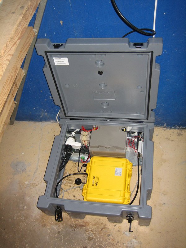
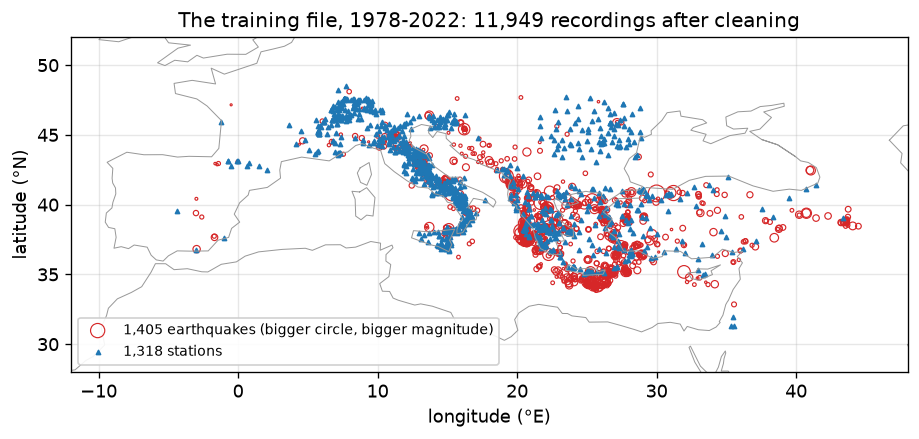
Left: a strong-motion accelerograph in a basement. Photo: EERC (public domain), via Wikimedia Commons. Right: drawn from your training file.

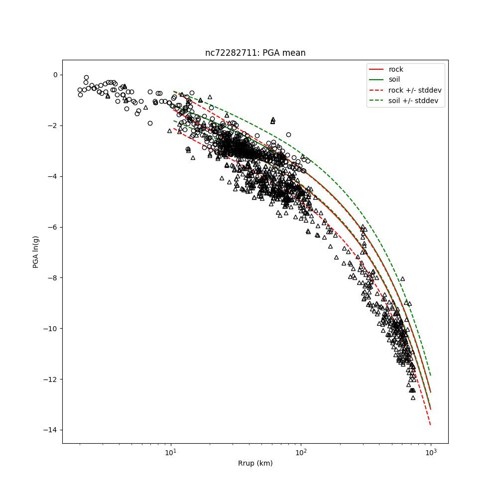
Researchers have built these models for decades, and four studies set up what you will try. The figure below is the model inside the Napa ShakeMap: the observations (circles and triangles; the plot does not say what each symbol means) against distance, with the model's curves for rock and soil. It falls with distance, as your models will, and the observations scatter widely around it.
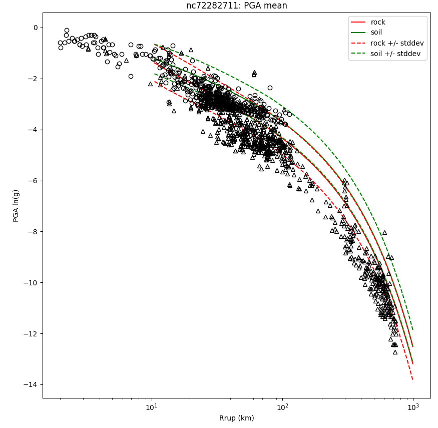
ln PGA against distance to the fault (log scale), 2014 South Napa. USGS ShakeMap (public domain).
- Atkinson (2006) compared 21 stations in Los Angeles: one station's recordings scatter less around the model than all the stations' together, because each station's ground repeats from one earthquake to the next (doi). That is the idea behind your station corrections.
- Kotha and colleagues (2020) fitted a model to the ESM data to update Europe's seismic hazard and risk assessment, with corrections for 1,829 stations (doi). You will score their published equation.
- Kubo and colleagues (2020) found that a machine-learning model predicted the strongest shaking too low, because strong recordings are rare in the data; adding a conventional equation reduced it (doi). Watch what your random forest does at the largest magnitudes.
- Okazaki and colleagues (2021) showed that a flexible model can fit the stations it was trained on and miss new ones, so how the data are split decides whether a test is fair (doi).
The largest earthquakes matter most and are the rarest in the data, so predicting them is still open. In 45 years the training file holds 256 recordings of magnitude 7 or more, from 7 earthquakes. The leaderboard's recordings since 2023 hold 212. In this project you build a model step by step, test it fairly on earthquakes it has never seen, try a freer model and a correction for each station, and enter your best on a leaderboard scored on those 2023 recordings.
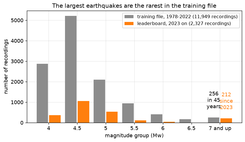
Drawn from the training file and the leaderboard's inputs.
What you'll be able to do
The science. Say how hard the ground shakes at a distance from an earthquake of a given magnitude, why the shaking stops growing as fast for the largest earthquakes, why soft ground shakes harder than rock, and why each station shakes in its own way.
The code. You write every line: a scatter plot coloured by a column, a function for the
typical miss, LinearRegression on columns you make, a mean for each group, a split by time, a
bootstrap over whole earthquakes, RandomForestRegressor, a correction for each station chosen on
a fair test, and a submission.csv file.
The four questions of the project:
- How does the shaking fade with distance, and grow with magnitude?
- Can an equation in magnitude and distance predict the shaking?
- How well does the equation do on earthquakes it has never seen?
- Does a more flexible model, or more information, do better on new earthquakes?
What you hand in, and when
One Gradescope assignment, "Final project: ground motion", takes everything.
- Individual work. Start now; Gradescope takes uploads from Wed 25 Nov, and the project is due Wed 16 Dec. Mon 7 Dec (RRR week) has no class, but you are welcome to come to the room in class time and work on your notebook.
- Every upload carries two files:
submission.csv(your leaderboard entry, made by the last Your turn) and this notebook. Gradescope cannot check this for you, so follow these steps:- In DataHub, save the notebook (File ▸ Save).
submission.csvis in the same folder as the notebook, in the left-hand panel. - Download both: right-click each file in the left-hand panel and choose Download.
- In Gradescope, open Final project: ground motion, click Upload Submission, and select both files (hold Ctrl, or Cmd on a Mac, to select the second), or drag both into the window. Type a name for the leaderboard: your own name or a nickname. Your classmates will see it next to your score.
- Check that Gradescope lists both files, then upload. If the result says a file is missing, upload both again.
- In DataHub, save the notebook (File ▸ Save).
- Up to 10 uploads that change
submission.csvare scored on the leaderboard. An upload that changes only the notebook is free. - Everything is due Wed 16 Dec at 23:59 Pacific time: the notebook and your last entry.
- Before every upload: Kernel → Restart Kernel and Run All Cells must run from top to bottom without an error.
How it is graded (100 points). The Your turns are graded like a week's. The leaderboard gives two grades: one for a valid entry that beats always guessing the average, and one for your rank, on the final score from the hidden part of the board. Choose your entry by your own fair test, not by the public score.
| What | Points | Graded by | Full marks when |
|---|---|---|---|
| Your turns 1 to 12 | 80 | Gradescope, when you upload | each Your turn by its self-check (Your turn 1, a figure, for being done and run), and the notebook runs from top to bottom without an error |
| Leaderboard entry | 10 | Gradescope, pass or fail | your last submission.csv is valid and beats always guessing the average |
| Leaderboard rank | 10 | after the board closes | your final score, on the hidden part, ranked among the students on this project: top quarter 10, second quarter 8, third quarter 6, last quarter 4; a tie takes the higher band; no valid entry 0 |
Setup
Run the next two cells once. All their code is given. Three files from the ESM database (see the Background) ship with the course:
trackT1_esm_flatfile.csv.gz: every recording of an earthquake of about magnitude 4 or more, 1972 to 2022, your training file, downloaded on 7 November 2026 and frozen, so everyone trains on the same file;trackT1_leaderboard_test.csv: the leaderboard file, every recording from 1 January 2023 on, with the inputs and the station but not the shaking;trackT1_submission_template.csv: the empty submission template, one row per leaderboard recording.
import numpy as np
from sklearn.ensemble import RandomForestRegressor
from sklearn.linear_model import LinearRegression
import pandas as pd
import matplotlib.pyplot as plt

# house style, set once, so every plot cell below holds only what matters
plt.rcParams.update({"figure.figsize": (7, 4.5), "figure.dpi": 110,
                     "axes.grid": True, "grid.alpha": 0.3, "axes.axisbelow": True})

CACHE = "https://raw.githubusercontent.com/AI4EPS/EPS88_PyEarth/main/data"

# larger text, so every label and legend reads at a glance
plt.rcParams.update({"font.size": 11, "axes.titlesize": 12, "legend.fontsize": 9.5,
                     "legend.framealpha": 0.9})

records = pd.read_csv(CACHE + "/trackT1_esm_flatfile.csv.gz", sep=";")
leaderboard = pd.read_csv(CACHE + "/trackT1_leaderboard_test.csv")
template = pd.read_csv(CACHE + "/trackT1_submission_template.csv")
print("training file, as it arrives:", records.shape)
print("leaderboard file:", leaderboard.shape)
The next cell keeps the records a model can use, with the same rules that made the
leaderboard file: the peak ground acceleration (PGA) was measured and not flagged bad; magnitude 4
or more; depth 0 to 40 km; station within 200 km, with a known Vs30. Vs30 is the speed of shear
waves in the top 30 m of ground, in m/s: low for mud, high for rock. We predict ln_pga, the
natural log of the PGA in g (g = 981 cm/s², the pull of gravity). The cell also labels each
record with its magnitude_group, the magnitude rounded down to the half unit (5.3 goes in 5.0,
5.7 in 5.5), with everything from 7 up in 7.0.
# distance to the surface above the fault where known, else to the epicentre
records["distance_km"] = records["jb_dist"].fillna(records["epi_dist"])
records["pga_g"] = records["rotd50_pga"] / 981   # cm/s² to g

good = records[(records["pga_g"] > 0)
               & (records["quality_class"] != "BAD")
               & (records["late_triggered_event_01"].fillna(0) == 0)
               & (records["mw"] >= 4)
               & (records["ev_depth_km"] > 0)
               & (records["ev_depth_km"] < 40)
               & (records["distance_km"] <= 200)
               & records["preferred_vs30_m_s"].notna()]

# one table with the leaderboard file's column names, plus the answer and three labels
train = pd.DataFrame({"event_id": good["esm_event_id"],
                      "year": good["event_time"].str[:4].astype(int),
                      "station": good["network_code"] + "." + good["station_code"],
                      "Mw": good["mw"],
                      "distance_km": good["distance_km"],
                      "depth_km": good["ev_depth_km"],
                      "vs30_m_s": good["preferred_vs30_m_s"],
                      "ln_pga": np.log(good["pga_g"])}).reset_index(drop=True)
# the magnitude rounded down to the half unit, everything from 7 up in one group
train["magnitude_group"] = (np.floor(train["Mw"] * 2) / 2).clip(upper=7)

print("recordings a model can use:", len(train))
print("earthquakes:", train["event_id"].nunique(), "  stations:", train["station"].nunique())
print("years:", train["year"].min(), "to", train["year"].max())
print(train.head())
1. How does the shaking fade with distance, and grow with magnitude?
We work with the log of the PGA. PGA is quoted as a fraction of g, the pull of gravity: a
PGA of 1 g pushes sideways as hard as gravity pulls down. In the training file it runs from
0.000008 g far from a small earthquake to 0.83 g beside a large one, a
range of about 100,000 times. Its natural log, ln_pga, runs from
-11.7 to -0.2, and a change of 1 in ln_pga is a factor
of e, about 2.7, at any size. To read the plots: ln_pga of −1 is 0.37 g, −3 is
0.05 g, and −6 is 0.0025 g.
How much weaker is the shaking far away, and how much do stations at the same distance differ? The next cell draws every recording of the earthquake with the most recordings in the file, against the station's distance, with the median near and far marked.
# the earthquake with the most recordings, sorted by distance
busiest_id = train["event_id"].value_counts().index[0]
one_quake = train[train["event_id"] == busiest_id].sort_values("distance_km")
close_by = one_quake[one_quake["distance_km"] < 10]["ln_pga"]
far_away = one_quake[one_quake["distance_km"] > 80]["ln_pga"]

plt.figure(figsize=(8, 4.5))
plt.scatter(one_quake["distance_km"], one_quake["ln_pga"], s=14, color="0.3", label="one station")
plt.hlines(np.median(close_by), 0, 10, color="tab:red", lw=4, label="median within 10 km")
plt.hlines(np.median(far_away), 80, 102, color="tab:blue", lw=4, label="median beyond 80 km")
plt.axvspan(45, 55, color="gold", alpha=0.3, label="45-55 km: one distance, many values")
plt.xlabel("distance to the earthquake (km)")
plt.ylabel("ln PGA (g)")
plt.title(f"Earthquake {busiest_id}, Mw {one_quake['Mw'].iloc[0]}: {len(one_quake)} stations")
plt.legend()
plt.show()
Far stations shook about 7 times less than near ones,
and stations at one distance still differ by a factor of 4. This
magnitude 7.7 earthquake struck Taiwan in 1999. The median ln_pga is
-1.7 within 10 km (red) and -3.7 beyond 80 km (blue). The
30 stations between 45 and 55 km (yellow band) span 1.3 in
ln_pga, because the ground under each one differs. A model will not remove that scatter; it
describes the trend through it.
✏️ Your turn 1
What do all 11,949 recordings look like, near and far, small and large?
Why: before any model, look at the data. One earthquake showed the fading with distance; all of them together show what magnitude adds.
Look back at: the scatter plot coloured by a column, from Where do earthquakes and volcanoes
happen? (04_where_and_why.ipynb).
- Sort
trainbyMw, so the rare large earthquakes are drawn last, on top of the small ones. - Draw a scatter plot of
ln_pga(up) againstdistance_km(across) for every row, with small dots (s=2), each coloured by its magnitude,Mw. - Add a colour bar labelled with what the colour means.
- Label both axes with their units, and give the plot a title with the number of recordings.
This Your turn has no self-check: a figure you can see needs none. A good figure shows, at a glance, the cloud falling from left to right and the large earthquakes as a bright band on top. Check it yourself: the title says 11,949, and the colour bar runs from magnitude 4 to above 8.
# ← your answer here: write your code here
Shaking fades with distance, and the large earthquakes (yellow) sit on top. Between 40 and
60 km, the median ln_pga is -6.3 for magnitude 4 to 4.5 and -3.0
for magnitude 6 and up: a factor of about 25. Most dots
are dark: small earthquakes are common, and large ones rare.
Think. If you had to guess one number for every recording, knowing nothing about it, which number would you pick?
✏️ Your turn 2
How far off is the simplest guess: the same number for every recording?
Why: this number is the bar that every model after it has to clear.
Baseline: Write the dumbest rule you can, first. Any model that cannot beat it is decoration.
Typical miss: Square every gap between what happened and what the curve said, average the squares, and take the square root: the usual size of a miss, in the data's own units.
Look back at: the typical miss, from When will CO2 pass 450 ppm? (07_co2_450_ppm.ipynb).
- Write a function
typical_miss(errors)that takes a column of errors and returns their typical miss. You will use it for every model in this notebook. - The rule: guess the average
ln_pgaof all the training recordings. Name itaverage_ln_pga. - Each recording's error is its
ln_pgaminus that guess. Their typical miss isbaseline_miss. - Print the guess, the typical miss, and the factor it stands for (e to the power of the miss).
Use these names, because the self-check looks for them: typical_miss, average_ln_pga,
baseline_miss.
# ← your answer here: write your code here
# the self-check reads: typical_miss, average_ln_pga, baseline_miss
# Self-check: run this after your answer. You do not need to read it — it only says whether something is off.
assert abs(typical_miss(np.array([3.0, -4.0])) - np.sqrt(12.5)) < 1e-9, \
    "the typical miss of the errors 3 and -4 is the square root of (9 + 16) / 2"
assert abs(average_ln_pga - (-6.5768)) < 0.001, \
    "the guess is the average ln PGA of the training recordings"
assert abs(baseline_miss - 1.9024) < 0.002, \
    "the typical miss of each recording's ln PGA minus that average"
print(f"✓ Your turn 2 — always guessing {average_ln_pga:.2f} misses by {baseline_miss:.3f}")
Always guessing -6.58 misses by 1.90 in ln_pga: a factor of
6.7. A guess of 0.0014 g (e to the -6.58) is
typically wrong by 6.7 times, too high or too low. That is the bar: a model that cannot beat 1.90 has
learned nothing from magnitude and distance.
2. Can an equation in magnitude and distance predict the shaking?
Shaking grows with magnitude and fades with the log of distance. As waves spread out from the
earthquake, their energy is shared over a larger and larger sphere, so their size falls roughly as
one over the distance. In logs, a fall like that is a straight line in the log of the distance.
And each step of magnitude multiplies the energy released, so ln_pga rises roughly in a straight
line with magnitude. Together:
$$\ln \mathrm{PGA} = a + b\,M + c\,\ln r$$
- $M$ is the magnitude,
Mw; - $r$ is the distance in km, with 8 km added in the way of a right triangle,
$r = \sqrt{R^2 + 8^2}$, where $R$ is
distance_km. The earthquake starts several km under the ground, so even a station right above it is not at distance 0, and $\ln 0$ does not exist; - $a$, $b$ and $c$ are three numbers that linear regression finds.
Linear regression: Draw the best straight line. Best means the smallest root mean squared error: the line that misses its points least.
With two columns it finds the best flat surface instead of a line, in the same way.
✏️ Your turn 3
How close does a straight line in magnitude and log distance get?
Why: this is the simplest model with any physics in it. Each improvement after it has to beat it.
Look back at: LinearRegression, from How old is the universe? (06_age_of_the_universe.ipynb).
- Add the column
ln_distancetotrain: $\ln r$, the log of √(distance_km² + 8²). - Fit a
LinearRegressionofln_pgaon the two columnsMwandln_distance, for every training recording. Name itline. - Bind its numbers to the equation's symbols:
ais the intercept, andbandcare the two coefficients, in the order of the columns. Print the equation with them. - Add the line's prediction for every recording as the column
lineoftrain. line_miss: the typical miss ofln_pgaminus that prediction. Print it besidebaseline_miss.
Use these names, because the self-check looks for them: line, a, b, c, line_miss.
# ← your answer here: write your code here
# the self-check reads: line, a, b, c, line_miss
# Self-check: run this after your answer. You do not need to read it — it only says whether something is off.
assert abs(b - 1.2198) < 0.002, "b: how much ln PGA rises for one step of magnitude"
assert abs(c - (-1.8491)) < 0.002, "c: how much ln PGA changes for one step of ln r, with 8 km in r"
assert abs(line_miss - 0.9793) < 0.002, "the typical miss of ln PGA minus the line's prediction"
print(f"✓ Your turn 3 — ln PGA = {a:.2f} + {b:.2f} M + {c:.2f} ln r, typical miss {line_miss:.3f}")
Does the line follow the data at each magnitude? The next cell draws the fitted equation for three magnitudes, over the recordings within a quarter unit of each, with the two typical misses written on the plot.
# line, a, b and c: the fit of Your turn 3; one curve per magnitude, over the recordings near it
distances = np.arange(0, 201, 2)
ln_r = np.log(np.sqrt(distances ** 2 + 8 ** 2))

plt.figure(figsize=(8, 5))
for magnitude, colour in [(4.5, "tab:blue"), (5.5, "tab:orange"), (6.5, "tab:red")]:
    near = train[(train["Mw"] > magnitude - 0.25) & (train["Mw"] <= magnitude + 0.25)]
    plt.scatter(near["distance_km"], near["ln_pga"], s=3, color=colour, alpha=0.3)
    plt.plot(distances, a + b * magnitude + c * ln_r, color=colour, lw=2.5,
             label=f"M {magnitude}: line, and {len(near)} recordings")
plt.text(110, 1.2, f"typical miss\n  line: {line_miss:.2f}\n  always the average: {baseline_miss:.2f}",
         va="top")
plt.ylim(-12.5, 1.8)   # room above the curves for the text
plt.xlabel("distance to the earthquake (km)")
plt.ylabel("ln PGA (g)")
plt.title(f"ln PGA = {a:.2f} {b:+.2f} M {c:+.2f} ln r, fitted to {len(train)} recordings")
plt.legend(loc="lower left")
plt.show()
The line halves the miss: 0.98 against 1.90 for always the
average. Each step of magnitude adds 1.22 to ln_pga, a factor of
3.4, and the curves follow the clouds of dots. But the line treats every
magnitude the same way. Does it miss some magnitudes more than others?
Residual: A residual is the real value minus the line's value.
Here, a recording's residual is its ln_pga minus the
model's prediction: above zero, the ground shook harder than the model said.
✏️ Your turn 4
Does the line miss small and large earthquakes in the same way?
Why: a good model's residuals average zero at every magnitude. If one group sits above zero, the model is too low for it, and the shape of the equation is wrong there.
Look back at: groupby, from Earth's elevation has two peaks (03_two_peaks.ipynb).
- Write a function
mean_by_magnitude(column)that takes the name of a column oftrainand returns its mean in eachmagnitude_group. - Add the column
line_residualtotrain:ln_pgaminus the line's prediction. line_by_magnitude:mean_by_magnitudeof that column. Print it, rounded to 2 places.- Plot it: the mean residual (up) against the magnitude group (across), as dots joined by a line,
with a horizontal line at zero. Write each group's value beside its dot, with a loop over the
groups and
plt.text(x, y, words). Label both axes and give a title. A good figure shows at a glance which magnitudes the line misses, and by how much.
Use these names, because the self-check looks for them: mean_by_magnitude,
line_by_magnitude.
# ← your answer here: write your code here
# the self-check reads: mean_by_magnitude, line_by_magnitude
# Self-check: run this after your answer. You do not need to read it — it only says whether something is off.
assert abs(mean_by_magnitude("ln_pga")[4.0] - (-7.2277)) < 0.001, \
    "the mean of the column over the recordings in each magnitude group"
assert abs(line_by_magnitude[5.5] - 0.4611) < 0.005, \
    "for each magnitude group, the mean of ln PGA minus the line's prediction"
print(f"✓ Your turn 4 — the line is {line_by_magnitude[5.5]:+.2f} off at magnitude 5.5 to 6")
The line is too low for magnitudes 5.5 to 6.5, and far too high from 7 up. Recordings of
magnitude 5.5 to 6 shook +0.46 harder than the line said (a factor of
1.6); those of magnitude 7 and up, from 7 earthquakes, shook
1.17 less in ln_pga than the line said, a factor of 3.2. A
straight line in magnitude cannot bend, and the data bend over at the top.
The physics says how to bend it. Ground-motion models add columns for four effects:
- Big earthquakes stop getting stronger as fast (saturation): a large earthquake breaks a fault tens of km long, and a station is near only part of it. A term in $M^2$ lets the rise bend.
- Big earthquakes fade more slowly with distance, for the same reason: a column $M \ln r$ lets the distance slope change with magnitude.
- Rock absorbs a little energy every km, on top of the spreading: a column in the distance itself, $R$.
- Soft ground shakes harder than rock: waves slow down in mud and grow taller. A column $\ln V_{s30}$.
$$\ln \mathrm{PGA} = a + b_1 M + b_2 M^2 + c_1 \ln r + c_2 M \ln r + c_3 R + d \ln V_{s30}$$
It is still linear regression: each term is a column times a number, so LinearRegression finds
the seven numbers just as it found three. In Python the new columns are Mw_squared ($M^2$),
Mw_ln_distance ($M \ln r$) and ln_vs30 ($\ln V_{s30}$); $R$ is distance_km.
✏️ Your turn 5
Does the six-column equation miss less, and miss every magnitude more evenly?
Why: each new column stands for a piece of physics. If the physics is right, the typical miss falls and the residuals by magnitude move toward zero.
Look back at: your Your turns 3 and 4.
- Add three columns to
train:Mw_squared,Mw_ln_distanceandln_vs30, as named in the cell above. six_columns: a list of the six column names,Mw,Mw_squared,ln_distance,Mw_ln_distance,distance_km,ln_vs30.- Fit a
LinearRegressionofln_pgaon them, for every training recording. Name itequation, and add its prediction as the columnequationoftrain. equation_miss: its typical miss. Print it besideline_miss.- Add the column
equation_residual, andequation_by_magnitude: yourmean_by_magnitudeof it. Print it in a table besideline_by_magnitude, rounded to 2 places.
Use these names, because the self-check looks for them: six_columns, equation,
equation_miss, equation_by_magnitude.
# ← your answer here: write your code here
# the self-check reads: six_columns, equation, equation_miss, equation_by_magnitude
# Self-check: run this after your answer. You do not need to read it — it only says whether something is off.
assert sorted(six_columns) == sorted(["Mw", "Mw_squared", "ln_distance", "Mw_ln_distance", "distance_km", "ln_vs30"]), \
    "the six columns named in the prompt"
assert abs(equation_miss - 0.9092) < 0.002, \
    "the typical miss of ln PGA minus the six-column equation's prediction"
assert abs(equation_by_magnitude[5.5] - 0.2396) < 0.005, \
    "for each magnitude group, the mean of ln PGA minus the equation's prediction"
print(f"✓ Your turn 5 — typical miss {equation_miss:.3f}; {equation_by_magnitude[5.5]:+.2f} off at magnitude 5.5 to 6")
Did the physics pull every magnitude toward zero? The next cell draws both sets of residuals, with a grey band for a miss smaller than 0.1 either way.
# line_by_magnitude and equation_by_magnitude: Your turns 4 and 5
plt.figure(figsize=(8, 4.5))
plt.axhspan(-0.1, 0.1, color="0.88", label="within 0.1 of zero")
plt.plot(line_by_magnitude.index, line_by_magnitude.values, "o-", color="tab:blue",
         label=f"straight line, 2 columns: typical miss {line_miss:.2f}")
plt.plot(equation_by_magnitude.index, equation_by_magnitude.values, "s-", color="tab:red",
         label=f"equation, 6 columns: typical miss {equation_miss:.2f}")
plt.axhline(0, color="k", lw=1)
for residuals, colour in [(line_by_magnitude, "tab:blue"), (equation_by_magnitude, "tab:red")]:
    plt.text(7.05, residuals[7.0], f"{residuals[7.0]:+.2f}", color=colour)
plt.xlabel("magnitude group (Mw, rounded down to the half unit)")
plt.ylabel("mean residual (ln PGA)")
plt.title(f"Residuals by magnitude, {len(train)} recordings")
plt.legend(loc="lower left")
plt.show()
The equation misses less, 0.91 against 0.98, and more evenly. At magnitude 5.5 to 6 its residuals average +0.24, against +0.46 for the line; from 7 up, -0.20 against -1.17. Its worst group is 0.24 from zero, against 1.17. The physics in the extra columns was in the data.
But both numbers are scores on the recordings the models were fitted to. A model can fit the recordings it has seen and still miss the next earthquake. The leaderboard asks about the next earthquakes, so the next section asks the same.
3. How well does the equation do on earthquakes it has never seen?
A model is judged on data it did not learn from, as in the CO2 week.
Train/test split: Hide some data from yourself, then check.
But which recordings to hide? A random choice of rows would be unfair here, because the recordings of one earthquake miss together: an earthquake that shook harder than its magnitude says shook harder at every station. The next cell shows it for the five best-recorded earthquakes.
# the equation's residuals (Your turn 5), averaged over each of the five best-recorded earthquakes
best_recorded = train["event_id"].value_counts().index[:5]
for quake in best_recorded:
    its_records = train[train["event_id"] == quake]
    print(quake, " Mw", its_records["Mw"].iloc[0], " recordings:", len(its_records),
          " mean residual:", round(np.mean(its_records["equation_residual"]), 2))
Each earthquake has its own offset, from -0.27 to +1.31 among these five. If some of an earthquake's recordings were in the training rows and the rest hidden, the model would have learned that earthquake's offset from the first, and the test would be too kind. So we hide whole earthquakes: we split by structure, not at random. The leaderboard does the same by time: it trains on everything before 2023 and tests on what came after. We copy it: fit on the earthquakes before 2018, test on 2018 to 2022.
✏️ Your turn 6
How far off is the equation on earthquakes it has never seen?
Why: this is the number that predicts how your model will do on the leaderboard. The score on fitted recordings does not.
Look back at: the split by time, from When will CO2 pass 450 ppm? (07_co2_450_ppm.ipynb).
fit_part: the rows oftrainfrom before 2018.hidden_part: the rows from 2018 on (take a.copy(), because you will add columns to it). Print how many recordings and earthquakes each holds.- Fit the six-column equation on
fit_partonly. Name itequation_before. - Add its prediction for each hidden recording as the column
equationofhidden_part. test_miss: the typical miss on the hidden recordings. Print it besideequation_miss.
Use these names, because the self-check looks for them: fit_part, hidden_part,
test_miss.
# ← your answer here: write your code here
# the self-check reads: fit_part, hidden_part, test_miss
# Self-check: run this after your answer. You do not need to read it — it only says whether something is off.
assert len(hidden_part) == 4643 and hidden_part["year"].min() == 2018, \
    "the hidden part is every recording from 2018 on"
assert len(fit_part) + len(hidden_part) == len(train), "every recording is in exactly one part"
assert abs(test_miss - 0.9577) < 0.002, \
    "fit on the part before 2018; the typical miss of the hidden ln PGA minus its prediction"
print(f"✓ Your turn 6 — the equation misses the hidden earthquakes by {test_miss:.3f}")
On new earthquakes the equation misses by 0.958, more than the 0.909 it scored on the recordings it was fitted to. That is normal, and it is why the fitted score is never the one to report. The hidden part holds 515 earthquakes. A different 515 would give a slightly different miss. How different?
Bootstrap: Ask the data the same question a thousand times, using a different random slice of itself each time.
Here the slice must be whole earthquakes, because their recordings miss together. A simple case first: three earthquakes, A recorded by four stations, B by two and C by one. The next cell writes down, for each earthquake, its number of recordings and the sum of their squared errors. A redraw picks three earthquakes with replacement, so one may come twice and another not at all, and its typical miss is the square root of (all the squared errors it holds ÷ all the recordings it holds).
# three made-up earthquakes: one row per recording, with that recording's squared error
toy = pd.DataFrame({"event_id": ["A", "A", "A", "A", "B", "B", "C"],
                    "squared_error": [0.1, 0.2, 0.1, 0.2, 1.5, 1.3, 0.4]})
toy["records"] = 1

# one row per earthquake: the sum of its squared errors, and its number of recordings
toy_per_quake = toy.groupby("event_id")[["squared_error", "records"]].sum()
print(toy_per_quake)
print("typical miss of all seven:", round(np.sqrt(np.sum(toy_per_quake["squared_error"])
                                                   / np.sum(toy_per_quake["records"])), 3))

# one redraw: three earthquakes, with replacement
toy_redraw = toy_per_quake.sample(3, replace=True, random_state=np.random.default_rng(1))
print(toy_redraw)
print("typical miss of this redraw:", round(np.sqrt(np.sum(toy_redraw["squared_error"])
                                                     / np.sum(toy_redraw["records"])), 3))
This redraw picked B, B, C, and its typical miss is 1.10 against 0.74 for the three as they are. Each earthquake came with all its recordings. A thousand redraws give a thousand typical misses, and their middle 95% is the interval: how much the score could move with other earthquakes like these.
✏️ Your turn 7
How much could the test score move with other earthquakes like these?
Why: two models whose scores differ by less than this are not clearly different. You will need the interval to judge every comparison from here on.
Look back at: the bootstrap, from How long was the Earth frozen? (08_how_long_frozen.ipynb),
and the three earthquakes just above.
- Add two columns to
hidden_part:squared_error, each recording's (ln_pga− the equation's prediction)², andrecords, 1 on every row. per_quake: one row per earthquake, the sums of those two columns, as in the simple case.- Make a random generator,
rng = np.random.default_rng(88), and an empty list,redrawn_misses. - 1,000 times: redraw as many earthquakes as
per_quakeholds, with replacement (random_state=rng), and append the redraw's typical miss. test_interval: the 2.5th and 97.5th percentiles of the 1,000 misses. Print it besidetest_miss.- Draw a histogram of the 1,000 misses, with vertical lines at the two ends of the interval and
at
test_miss, each with its number in the legend, so the figure says how wide the interval is without a printout.
Use these names, because the self-check looks for them: per_quake, redrawn_misses,
test_interval.
# ← your answer here: write your code here
# the self-check reads: per_quake, redrawn_misses, test_interval
# Self-check: run this after your answer. You do not need to read it — it only says whether something is off.
assert len(per_quake) == 515 and per_quake["records"].sum() == 4643, \
    "one row per hidden earthquake, holding its number of recordings"
assert abs(np.mean(redrawn_misses) - 0.9581) < 0.005, \
    "each redraw's typical miss: the square root of its squared errors summed over its recordings"
assert abs(test_interval[0] - 0.9187) < 0.01 and abs(test_interval[1] - 1.0028) < 0.01, \
    "the 2.5th and 97.5th percentiles of 1,000 redraws of whole earthquakes"
print(f"✓ Your turn 7 — 95% interval {test_interval[0]:.3f} to {test_interval[1]:.3f}")
The equation's test miss is 0.958, with a 95% interval from 0.919 to 1.003. The interval is 0.08 wide. So a new model that scores, say, 0.01 better on these hidden earthquakes has not clearly beaten the equation: other earthquakes could reverse the order. A model that lands below 0.92 would have.
4. Does a more flexible model, or more information, do better on new earthquakes?
There are two ways to try to beat the equation. One is a more flexible model, free to find any shape in the data. The other is more information: something about each recording that the six columns do not hold. This section tries both, on the same hidden earthquakes.
A random forest learns its shape from the data, not from an equation. You met it in the basalt week, where its trees voted for a setting.
Random forest: Ask many slightly different trees and take a vote.
For a number instead of a label, RandomForestRegressor averages its trees' answers instead of
taking a vote.
How a random forest decides, in one picture:
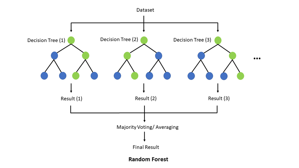
Many decision trees each give an answer; a forest that predicts a number averages them. Each tree is grown on its own bootstrap sample. Figure: TseKiChun (CC BY-SA 4.0), via Wikimedia Commons.
It needs no made-up columns: a tree can cut distance_km anywhere, so it is given the four
inputs as they are, Mw, distance_km, depth_km and vs30_m_s. But a tree can only predict
values like those in its leaves, and large earthquakes are rare: 48 of the
890 earthquakes in fit_part are magnitude 6 or more.
✏️ Your turn 8
Does a random forest beat the equation on the hidden earthquakes?
Why: the forest is free to find any shape the data show. If the equation's shape is missing something, the forest should do better.
Look back at: the random forest, from Where was this basalt made? (10_where_basalt.ipynb).
four_inputs: the listMw,distance_km,depth_km,vs30_m_s.forest: aRandomForestRegressor, fitted onfit_part's four inputs andln_pga, for example withn_estimators=100, min_samples_leaf=5, random_state=0(min_samples_leaf=5keeps at least five recordings in each leaf, so no tree learns one station by heart). Other settings are fine.- Add its prediction for each hidden recording as the column
forestofhidden_part. forest_test_miss: the typical miss on the hidden recordings, with yourtypical_miss. Print it besidetest_missandtest_interval; it should sit far belowbaseline_miss.
Use these names, because the self-check looks for them: forest, forest_test_miss.
# ← your answer here: write your code here
# the self-check reads: forest, forest_test_miss
# Self-check: run this after your answer. You do not need to read it — it only says whether something is off.
assert hasattr(forest, "predict") and "forest" in hidden_part, \
    "forest is a fitted model, and hidden_part has a column forest with its prediction for each hidden recording"
assert abs(forest_test_miss - typical_miss(hidden_part["ln_pga"] - hidden_part["forest"])) < 1e-6, \
    "forest_test_miss is the typical miss of the hidden ln PGA minus the forest column"
assert 0.9 * test_miss < forest_test_miss < baseline_miss, \
    "the forest's miss on the hidden earthquakes is out of range: was it fitted on the fitting part only, and on ln PGA?"
print(f"✓ Your turn 8 — the forest misses the hidden earthquakes by {forest_test_miss:.3f}, the equation by {test_miss:.3f}")
What does each model predict for a bigger and bigger earthquake? The next cell asks both models about one made-up site, 20 km from earthquakes of magnitude 4 to 8, over the fitting recordings at 15 to 25 km. The grey band marks where the forest's curve has gone flat: from there to magnitude 8 it stays within 0.1 of its value at 8.
# forest and equation_before: Your turns 8 and 6; one made-up site, at every magnitude from 4 to 8
site = pd.DataFrame({"Mw": np.arange(4, 8.01, 0.1)})
site["distance_km"] = 20
site["depth_km"] = 10
site["vs30_m_s"] = 400
site["ln_distance"] = np.log(np.sqrt(site["distance_km"] ** 2 + 8 ** 2))
site["Mw_squared"] = site["Mw"] ** 2
site["Mw_ln_distance"] = site["Mw"] * site["ln_distance"]
site["ln_vs30"] = np.log(site["vs30_m_s"])
site["equation"] = equation_before.predict(site[six_columns])
site["forest"] = forest.predict(site[four_inputs])

# the forest is flat from the first magnitude after which it stays within 0.1 of its value at 8
still_rising = site[np.abs(site["forest"] - site["forest"].iloc[-1]) > 0.1]
flat_from = np.max(still_rising["Mw"]) + 0.1

near = fit_part[(fit_part["distance_km"] >= 15) & (fit_part["distance_km"] <= 25)]
plt.figure(figsize=(8, 4.5))
plt.axvspan(flat_from, 8, color="0.9", label=f"the forest is flat from M {flat_from:.1f}")
plt.scatter(near["Mw"], near["ln_pga"], s=5, color="0.55", label=f"{len(near)} fitting recordings, 15-25 km")
plt.plot(site["Mw"], site["equation"], color="tab:red", lw=2.5, label="equation: keeps rising")
plt.plot(site["Mw"], site["forest"], color="tab:green", lw=2.5, label="forest")
plt.xlabel("magnitude, Mw")
plt.ylabel("ln PGA (g)")
plt.title("One site 20 km away: what each model predicts as magnitude grows")
plt.legend(loc="lower right")
plt.show()
The forest misses by 0.977, more than the equation's 0.958: its freedom
bought nothing on new earthquakes. The picture shows why. The forest's curve is a staircase that
follows the scatter of a few earthquakes, where the equation's shape comes from physics. And from
about magnitude 5.8 up, where fit_part holds only 75 earthquakes, the
forest stops rising (-2.42 at 5.8, -2.42 at 8): a tree can only
answer with an average of the recordings in its leaves, so it gives a magnitude 8 the shaking of a
5.8. The equation keeps rising, more slowly at the top (-2.90 to
-1.72), as the physics says.
At the largest magnitudes this picture shows the equation predicting too much, not the forest
too little. The 14 dots from magnitude 7 up have a median ln_pga of
-2.32, near the forest's flat line; 13 of them sit below the
equation. They come from very few earthquakes, so whether any model gets the largest earthquakes
right is the question this project ends on. The next try is not a freer shape, but more
information.
Every recording was made at a station, and each station sits on its own ground (Atkinson's idea, in the Background). Vs30 is one number for the top 30 m; the layers below, the shape of a valley, the hill a station stands on, all change the shaking too. If they make a station shake harder than the equation says, it does so for every earthquake. The next cell shows it for the five stations with the most recordings, with the equation's residuals from Your turn 5.
# the equation's residuals (Your turn 5), averaged over each of the five busiest stations
busiest_stations = train["station"].value_counts().index[:5]
for station in busiest_stations:
    its_records = train[train["station"] == station]
    print(station, " recordings:", len(its_records), " earthquakes:", its_records["event_id"].nunique(),
          " mean residual:", round(np.mean(its_records["equation_residual"]), 2))
Each station has its own offset, from -0.74 to -0.03 among these five,
over many earthquakes. That is information the six columns do not hold: a station's
correction, the equation's average miss there. The leaderboard file gives each recording's
station, and 74% of its recordings were made at a station that is also in
the training file. A station never seen before gets a correction of 0: the equation alone.
A simple case first. Three made-up stations: A with four recordings, B and C with one each.
The next cell finds each station's correction with groupby, and adds it to the equation's
prediction for three new recordings with .map(...), which looks each station up in the
corrections; .fillna(0) gives 0 to station D, which has none.
# three made-up stations: the equation's miss (ln PGA minus its prediction) at each of their recordings
toy_misses = pd.DataFrame({"station": ["A", "A", "A", "A", "B", "C"],
                           "miss": [0.5, 0.7, 0.4, 0.6, -0.9, 1.2]})
# a station's correction: the mean of its misses
toy_correction = toy_misses.groupby("station")["miss"].mean()
print(toy_correction)

# three new recordings: the equation's prediction plus the station's correction, 0 for D
toy_new = pd.DataFrame({"station": ["A", "C", "D"], "equation": [-4.0, -5.0, -3.0]})
toy_new["correction"] = toy_new["station"].map(toy_correction).fillna(0)
toy_new["with_correction"] = toy_new["equation"] + toy_new["correction"]
print(toy_new)
✏️ Your turn 9
Does each station's correction help on the hidden earthquakes?
Why: this is new information, not a new shape. If stations really shake in their own way, knowing each one's offset should cut the miss on earthquakes the model has never seen.
Look back at: groupby, from Earth's elevation has two peaks (03_two_peaks.ipynb), your Your
turn 6, and the three made-up stations just above.
- For each recording in
fit_part, its miss:ln_pgaminus the prediction ofequation_before(fitted onfit_part'ssix_columnsin Your turn 6). Keep it beside the recording'sstation. raw_correction: each station's mean miss, keyed by the station's name. Use onlyfit_part: the hidden recordings are the test.- For each hidden recording, the equation's prediction (the column
equationofhidden_part) plus its station's correction, with 0 for a station that is not infit_part. Keep the sum as a new column,raw_corrected, and leaveequationas it is: later cells read it. raw_fair_miss: the typical miss of the hiddenln_pgaminus that sum. Print it besidetest_missandtest_interval, and print what share of the hidden recordings were made at a station infit_part.
Use these names, because the self-check looks for them: raw_correction, raw_fair_miss.
# ← your answer here: write your code here
# the self-check reads: raw_correction, raw_fair_miss
# Self-check: run this after your answer. You do not need to read it — it only says whether something is off.
raw = pd.Series(raw_correction)
assert raw.index.isin(fit_part["station"]).all() and len(raw) == fit_part["station"].nunique(), \
    "raw_correction: one correction for each station in fit_part, keyed by its name, and none from the hidden part"
busiest = fit_part["station"].value_counts().index[0]   # the station with the most fitting recordings
its = fit_part[fit_part["station"] == busiest]
assert abs(raw[busiest] - np.mean(its["ln_pga"] - equation_before.predict(its[six_columns]))) < 0.01, \
    "a station's correction: the mean, over its recordings in fit_part, of ln PGA minus the equation's prediction"
assert 0.6 < raw_fair_miss < test_miss, \
    "with the corrections added, the hidden miss should fall below test_miss; check that a station that shook harder than the equation said makes its predictions higher, not lower"
print(f"✓ Your turn 9 — with station corrections {raw_fair_miss:.3f}, the equation alone {test_miss:.3f}")
With a correction for each station the equation misses the hidden earthquakes by 0.837,
against 0.958 alone: below the bottom of the interval, 0.919. That is a clear
win, from information rather than from a freer shape. 79% of the hidden
recordings were made at a station in fit_part; the rest got no correction.
But some of these corrections are guesses from one recording. Of the 1,081
stations in fit_part, 49% have a single recording. Its correction is
that one miss, which holds the station's ground but also the luck of that one earthquake. On the
fitting recordings the corrections cut the miss from 0.88 to 0.59,
far more than on the hidden ones.
Overfitting: A curve that memorises the data you gave it fails on the data you did not.
Here the corrections are what memorised: each fits its own station's recordings, luck included.
✏️ Your turn 10
At stations with only one fitting recording, do the corrections still help?
Why: a correction from one recording is the least certain. If anywhere the corrections are learning noise, it is there.
Look back at: value_counts, from the cells above, and your Your turn 9.
- Count the recordings of each station in
fit_part. thin: the hidden recordings whose station has exactly one recording infit_part. Print how many there are.thin_equation_miss: the typical miss onthinof the equation alone.thin_raw_miss: the typical miss onthinof the equation plus the raw corrections, the columnraw_correctedof Your turn 9. Print both.
Use these names, because the self-check looks for them: thin_equation_miss,
thin_raw_miss.
# ← your answer here: write your code here
# the self-check reads: thin_equation_miss, thin_raw_miss
# Self-check: run this after your answer. You do not need to read it — it only says whether something is off.
assert abs(thin_equation_miss - 0.9973) < 0.005, \
    "the typical miss of the equation alone, on the hidden recordings whose station has exactly one recording in fit_part"
assert abs(thin_raw_miss - 1.0358) < 0.005, \
    "the typical miss of the column raw_corrected, on the same hidden recordings"
assert thin_raw_miss > thin_equation_miss, \
    "at these stations the raw corrections should make the miss larger, not smaller"
print(f"✓ Your turn 10 — at one-recording stations: equation alone {thin_equation_miss:.3f}, with raw corrections {thin_raw_miss:.3f}")
At the 353 hidden recordings whose station had one fitting recording, the raw corrections make things worse: 1.036 against 0.997 for the equation alone. A one-recording correction copies one earthquake's luck, and the next earthquake does not share it.
The fix is to trust a correction only as far as its recordings allow. Instead of the mean, divide the sum of a station's misses by its number of recordings plus k:
$$\text{correction} = \frac{\text{sum of the station's misses}}{\text{its number of recordings} + k}$$
With k = 0 this is the mean. With k = 3, a station with one recording keeps a quarter of its miss, and one with 30 recordings keeps 30/33 of its mean: the correction shrinks toward 0 most where the evidence is thinnest. The next cell shows it on the three made-up stations.
# toy_misses: the three made-up stations above. Shrunk: the sum of the misses / (records + k)
toy_sums = toy_misses.groupby("station")["miss"].sum()
toy_counts = toy_misses.groupby("station")["miss"].count()
for k in [0, 1, 3]:
    print("k =", k, "  corrections:", (toy_sums / (toy_counts + k)).round(2).to_dict())
A has four recordings, so its correction shrinks least; B and C, with one each, shrink most. Which k is best is a question for the data. Choose it the way the CO2 week chose between models: try several, and compare their misses on years held back from the fit.
But treat small differences as ties. Your interval from Your turn 7 reaches about 0.04 either side of the miss, so two values of k whose misses differ by less than 0.01 are not clearly different. The cautious rule: among the k whose miss is within 0.01 of the smallest, choose the largest. It trusts each station's few recordings least, and gives up almost nothing on the fair test.
✏️ Your turn 11
Which k should the station corrections use?
Why: k sets how far to trust a station's few recordings. Too small and the corrections learn each earthquake's luck; too large and they shrink to nothing. The hidden earthquakes decide, and the cautious rule settles a tie.
Look back at: choosing between models on held-back months, from When will CO2 pass 450 ppm?
(07_co2_450_ppm.ipynb), and your Your turns 6 and 9.
- From the misses of Your turn 9, find each station's sum of misses and its number of
recordings in
fit_part. - Write a function that takes k and returns each station's shrunk correction, keyed by station.
- Try at least three values of k (0 among them is a good idea). For each, add the corrections to
the predictions in the hidden recordings'
equationcolumn, without changing that column (0 for a station not infit_part), and find the typical miss.miss_by_k: those misses, keyed by k (a dict or a Series). chosen_k: by the cautious rule, the largest k whose miss is within 0.01 of the smallest miss. (If you use another rule, say it in a comment.)station_correction: the corrections forchosen_k, keyed by station.fair_miss_with_corrections: its miss. Print them besideraw_fair_missandtest_miss.- Plot the miss (up) against k (across), with a horizontal line at
test_miss. A good figure also marks yourchosen_kand shades the band within 0.01 of the smallest miss (plt.axhspan), so a reader sees why the cautious rule chose it.
Use these names, because the self-check looks for them: miss_by_k, chosen_k,
station_correction, fair_miss_with_corrections.
# ← your answer here: write your code here
# the self-check reads: miss_by_k, chosen_k, station_correction, fair_miss_with_corrections
# Self-check: run this after your answer. You do not need to read it — it only says whether something is off.
tried = pd.Series(miss_by_k, dtype=float)
assert len(tried) >= 3, "miss_by_k: the hidden miss for at least three values of k"
assert chosen_k >= 0 and chosen_k in tried.index, "chosen_k: one of the values of k you tried, 0 or more"
ties = [k for k in tried.index if tried[k] <= tried.min() + 0.01]   # the k within 0.01 of the best
assert chosen_k == max(ties) or (chosen_k >= 1 and tried[chosen_k] < raw_fair_miss), \
    "chosen_k: by the cautious rule, the largest k whose miss is within 0.01 of the smallest (another rule must still give k of 1 or more that beats the raw corrections)"
assert abs(fair_miss_with_corrections - tried[chosen_k]) < 1e-6, "fair_miss_with_corrections: the miss at chosen_k"
shrunk, raw = pd.Series(station_correction), pd.Series(raw_correction)
records = fit_part["station"].value_counts()
two = records[records == 2].index[0]   # a station with two fitting recordings, where shrinking shows
assert abs(shrunk[two] - raw[two] * 2 / (2 + chosen_k)) < 0.005, \
    "station_correction: each station's sum of misses divided by (its number of recordings + chosen_k)"
assert 0.6 < fair_miss_with_corrections < test_miss and fair_miss_with_corrections <= raw_fair_miss + 0.005, \
    "the miss at chosen_k should be below the equation alone, and no worse than the raw corrections"
print(f"✓ Your turn 11 — k = {chosen_k}: typical miss {fair_miss_with_corrections:.3f}, raw {raw_fair_miss:.3f}, equation alone {test_miss:.3f}")
The smallest miss is 0.815, at k = 1; the k within 0.01 of it are 1, 2, 3, so the cautious rule chooses k = 3, with a miss of 0.822. That is 0.007 from the best, far inside the ±0.04 of the interval, against 0.837 for the raw corrections and 0.958 for the equation alone. Shrinking keeps what the busy stations know and quiets the guesses from one recording.
One caution. The hidden years have now been used to choose k, so this miss is a little kind to it.
Validation years: Years held back to choose between models. Once they have chosen, they are no longer a fair test.
The leaderboard, which nobody has used to choose anything, is the fair test of your final model.
The published model (Kotha et al. 2020, doi:10.1007/s10518-020-00869-1) is an equation like yours, with more physics in its shape. It adds three terms:
$$\ln \mathrm{PGA} = e_1 + f_R + f_M + f_S$$
- distance, $f_R$: a log-distance term whose slope changes with magnitude, and a straight term in distance, much as in your equation;
- magnitude, $f_M$: a curve up to a hinge magnitude, then a gentler straight line above it, because the largest earthquakes stop getting stronger as fast;
- ground, $f_S$: a curve in $\ln V_{s30}$.
Its numbers were fitted by its authors to an earlier release of this same database. The function
below is given: it returns the published model's ln_pga for every row of a table with
Mw, distance_km, depth_km and vs30_m_s.
def kotha_ln_pga(table, M_h=5.7):
    """Kotha et al. (2020), PGA, Vs30 version, no regional terms: ln PGA in g."""
    M = table["Mw"].values
    R = table["distance_km"].values
    depth = table["depth_km"].values
    vs30 = table["vs30_m_s"].values
    # the coefficients, as the open-source hazard software OpenQuake 3.26 prints them for PGA;
    # the paper's text puts the hinge M_h at 6.2, but these coefficients were fitted with it at 5.7
    e1 = 3.93782347219377
    b1, b2, b3 = 2.06573167101440, 0.304988012209292, 0.444773874960317
    c1, c2, c3 = -1.49787542346412, 0.281241474631338, -0.609876182476899
    g0, g1, g2 = -0.222196028066344, -0.558848724731566, -0.133014864040313
    # h: 4 km for an earthquake shallower than 10 km, 8 km to 20 km, 12 km below that
    h = np.where(depth < 10, 4.0, np.where(depth < 20, 8.0, 12.0))
    r = np.sqrt(R ** 2 + h ** 2)
    r_ref = np.sqrt(30 ** 2 + h ** 2)
    f_R = (c1 + c2 * (M - 4.5)) * np.log(r / r_ref) + c3 * (r - r_ref) / 100
    # below the hinge: a curve in M; above it: a gentler straight line
    f_M = np.where(M <= M_h, b1 * (M - M_h) + b2 * (M - M_h) ** 2, b3 * (M - M_h))
    f_S = g0 + g1 * np.log(vs30 / 800) + g2 * np.log(vs30 / 800) ** 2
    return e1 + f_R + f_M + f_S - np.log(981)   # the last term turns cm/s² into g
Which of the four models misses the hidden earthquakes least? The next cell is given: it scores the equation, the forest, the equation with your station corrections, and the published model, on all the hidden recordings and on those of magnitude 6 or more, and draws each beside the equation's interval.
# hidden_part: Your turns 6 and 8; station_correction: Your turn 11; kotha_ln_pga: the cell above
hidden_part["equation_and_stations"] = (hidden_part["equation"]
                                        + hidden_part["station"].map(pd.Series(station_correction)).fillna(0))
hidden_part["published"] = kotha_ln_pga(hidden_part)
big = hidden_part[hidden_part["Mw"] >= 6]
print("hidden recordings of magnitude 6 or more:", len(big), "from", big["event_id"].nunique(), "earthquakes")

models = ["equation", "forest", "equation_and_stations", "published"]
all_hidden = []
magnitude_6_up = []
for model in models:
    all_hidden.append(typical_miss(hidden_part["ln_pga"] - hidden_part[model]))
    magnitude_6_up.append(typical_miss(big["ln_pga"] - big[model]))
comparison = pd.DataFrame({"model": models, "all_hidden": all_hidden, "magnitude_6_up": magnitude_6_up})
print(comparison.round(3))

model_names = ["equation", "random forest", "equation + station corrections", "published (Kotha 2020)"]
plt.figure(figsize=(8, 3.5))
plt.axvspan(test_interval[0], test_interval[1], color="0.85", label="the equation's 95% interval")
plt.plot(all_hidden, range(len(models)), "o", color="firebrick", markersize=10)
for row, miss in enumerate(all_hidden):
    plt.text(miss, row + 0.2, f"{miss:.3f}", ha="center")
plt.yticks(range(len(models)), model_names)
plt.ylim(-0.5, len(models) - 0.3)
plt.xlabel("typical miss on the hidden earthquakes (ln PGA)\nsmaller is better")
plt.ylabel("model")
plt.title(f"Four models on {len(hidden_part)} hidden recordings, 2018-2022")
plt.legend(loc="lower left")
plt.show()
Only the station corrections clearly win: 0.822, below the interval, while the forest (0.977) and the published model (0.990) sit inside it with the equation (0.958). On the 143 recordings of magnitude 6 or more, from 15 earthquakes: the equation with station corrections 0.671, the equation 0.728, the published model 0.736, the forest 0.792. The better model came from better information about the physics, the ground under each station, and not from a fancier algorithm.
The leaderboard
leaderboard holds 2,327 recordings you have never seen, from 2023 on, up to
magnitude 7.7; 212 of them are magnitude 7 or more. It has the
input columns of train and the station (no event_id, year or ln_pga), plus row_id, the
key of each prediction. It also has three columns this notebook does not use: ec8_class (the
ground class of the European building code, from A for rock), fault_type (how the fault moved,
blank where unknown) and region (the station's country). They come from the raw training file's
preferred_ec8_code, fm_type_code and st_nation_code, so anyone who wants one can add it to
train. template has the same row_ids and an empty ln_pga column for your predictions.
- Your entry is your own model, fitted on the training file here. Do not look up or download the hidden answers (the recorded shaking of these 2023-on recordings, from ESM or anywhere else); a forecast built from them is not your model, and it scores 0.
- The board shows a public score on one third of the earthquakes below magnitude 7. The final score, on the other two thirds and on every recording of magnitude 7 or more, is shown after the board closes, and your rank on it is graded.
- So choose your entry by your own fair test, not by the public score. The public third is a few earthquakes; a model picked because it moved that number is tuned to them, and the rank uses the others.
- Up to 10 uploads that change
submission.csvare scored. An upload that changes only the notebook is free.
✏️ Your turn 12
Your leaderboard entry: how hard will the ground shake in 2,327 recordings from 2023 on?
Why: this is the project's answer, scored on shaking you have not seen, and ranked against the other students. Choose by your fair test: the public score is a third of the earthquakes, and your rank is decided on the rest.
Look back at: your Your turns 5, 9 and 11.
- Take the model your fair test chose: the six-column equation with station corrections shrunk by
your
chosen_k, unless your own tests found something better (the published model is not yours to enter). Make a freshfinal_model, and name its list of input columnsfinal_columns. - Fit it on every training recording: the hidden years are data too, and the newest.
final_correction: each station's shrunk correction, from the final model's misses on every training recording, keyed by station.- Add the same made columns (Your turns 3 and 5) to
leaderboard, made the same way. submission: a copy oftemplate, with itsln_pgacolumn filled with your model's prediction for each leaderboard recording plus its station's correction (0 for a station not intrain). Save it withsubmission.to_csv("submission.csv", index=False).- Print its first rows, its number of rows and of blanks, and the share of leaderboard recordings that got a correction.
- Run the self-check, then download
submission.csvand this notebook and upload both together (the steps are under "What you hand in" above) to Final project: ground motion.
Use these names, because the self-check looks for them: final_model, final_columns,
final_correction, submission.
# ← your answer here: write your code here
# the self-check reads: final_model, final_columns, final_correction, submission
# Self-check: run this after your answer. You do not need to read it — it only says whether something is off.
saved = pd.read_csv("submission.csv")
assert list(saved.columns) == ["row_id", "ln_pga"], "submission.csv holds the template's two columns, row_id and ln_pga"
assert (saved["row_id"].values == template["row_id"].values).all(), "one row per leaderboard recording, in the template's order"
assert saved["ln_pga"].notna().all(), "a prediction for every leaderboard recording"
assert np.allclose(saved["ln_pga"], submission["ln_pga"]), "submission.csv holds the table submission"
assert -12 < np.median(saved["ln_pga"]) < -1, "ln PGA in g, the log of the shaking, not the PGA itself"
assert final_model.n_features_in_ == len(final_columns), "the final model is fitted on its own input columns"
assert np.sqrt(np.mean((train["ln_pga"] - final_model.predict(train[final_columns])) ** 2)) < 1.2, \
    "the final model, fitted on every training recording, misses them by far less than always the average"
final = pd.Series(final_correction)
assert len(final) >= 0.95 * train["station"].nunique() and final.index.isin(train["station"]).all(), \
    "final_correction: one correction for each station in all of train, the hidden years included"
assert np.mean(np.abs(saved["ln_pga"] - final_model.predict(leaderboard[final_columns])) > 1e-6) > 0.5, \
    "the saved predictions should include each station's correction where the station is in train"
print(f"✓ Your turn 12 — submission.csv: {len(saved)} predictions, median ln PGA {np.median(saved['ln_pga']):.2f}")
The question, answered
On earthquakes it has never seen, an equation in magnitude, log distance and Vs30 predicts the
peak shaking within a typical factor of 2.6 (a miss of 0.96 in
ln_pga, against 1.90 for always the average); a random forest does no better,
but a shrunk correction for each station brings the miss down to about 0.82, a factor of
2.3. The equation's shape is the physics of how shaking grows and fades, so
here, on this split by time and these four inputs, a freer algorithm added nothing; what helped
was new information about the ground under each station.
The open question
Can a model you fit beat the published model on the largest earthquakes?
Your hidden years held 18 recordings of magnitude 7 or more, from 1 earthquake, so your fair test could not answer it. The leaderboard can: it holds the 2023 Türkiye earthquakes, and after the board closes it shows each student's final score on its 212 recordings of magnitude 7 or more, beside the published model's. Station corrections will not settle it alone: only 10 of those 212 recordings (5%) were made at a station in the training file, against 74% of all the leaderboard's recordings, so on the largest earthquakes your entry is mostly the equation itself. What would help where no station has recorded before is still an open question.