Is Mars's air thinning, or is Curiosity just climbing?
EPS 88 · PyEarth · final project. Open your own copy on DataHub: click here.
Since August 2012 the Curiosity rover has measured the air pressure on Mars every day. Year after year the readings come out lower. Is Mars losing its air? In this project you build a model of the pressure from Mars years 31 to 37 and use it to forecast 608 sols of Mars year 38, from its start to Ls 341. You never see the answers. The leaderboard does, and it ranks everyone's entries.
Background: what is going on with Mars's air?
1. A barometer on Mars reads less every year. Curiosity is a car-sized rover. It landed in Gale crater in August 2012, and its weather station has read the air pressure every day since. In its first Mars year (from 2012) its highest reading was 925 Pa; in its seventh (to 2024) the highest was 871 Pa, 6% less. Taken at face value, Mars is losing its air fast. This project finds out whether it is.
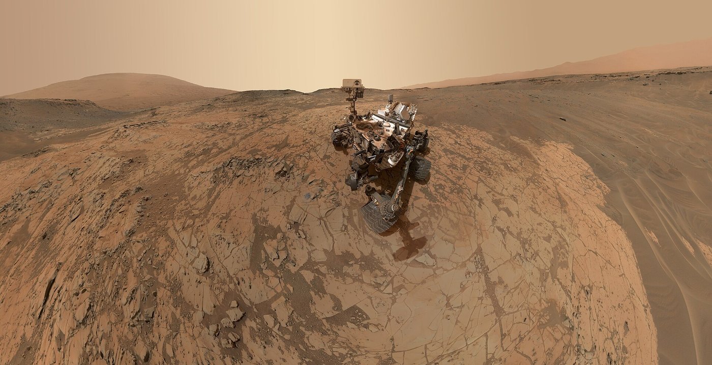
Curiosity on the lower slopes of Mount Sharp in January 2015: a self-portrait stitched from its arm camera, with the upper part of Mount Sharp on the horizon. NASA/JPL-Caltech/MSSS, PIA19142.
2. Mars's air is thin, and every winter part of it freezes. The median reading is 835 Pa, 0.8% of the air pressure at sea level on Earth (101,325 Pa). That air is almost all carbon dioxide (CO2). Over the pole that is in winter it gets cold enough for CO2 to freeze out of the air as frost on the polar cap; in spring the frost turns back into gas. So the pressure over the whole planet rises and falls with the seasons: in Mars year 32 Curiosity read from 732 to 925 Pa, a swing of 21%.
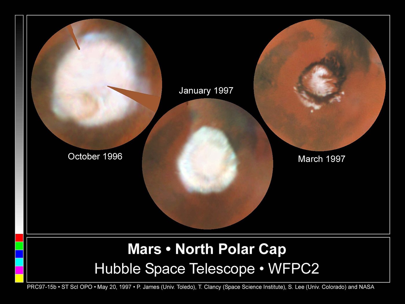
Mars's north polar cap seen by the Hubble Space Telescope, from early spring (October 1996) to the start of summer (March 1997): the CO2 frost turns back into air and the cap shrinks. P. James, T. Clancy, S. Lee and NASA/STScI, via Wikimedia Commons.

3. Why it matters: Mars did lose most of its air, but slowly. Early Mars was warmer than today. NASA's MAVEN orbiter measured gas escaping from the top of Mars's air to space at 2 to 3 kg every second, mostly hydrogen and oxygen atoms split from water, not the carbon dioxide of the air. Run back over Mars's history, escape removed at least about 0.8 bar of CO2 (96 times today's air), and it is the main reason Mars became cold and dry (Jakosky and others, 2018, doi:10.1016/j.icarus.2018.05.030). Today's air weighs about 32 million billion kg (its pressure times the area of Mars, divided by gravity). Even if all 3 kg per second came out of that air, escape would remove only 36 parts in a billion of it over Curiosity's 12 years: far too little to see. So the 6% drop is something else.
4. Three things move the barometer at once, and a model pulls them apart. The season moves it, through the polar caps. The rover's height moves it: Curiosity has been driving up Mount Sharp, a mountain about 5 km high in the middle of the crater, and climbed 848 m in these years; the higher you stand, the less air is above you. And the weather moves it, above all dust storms. You cannot tell the three apart by looking at the readings. A model with one part for each can measure each one, and you can test it by forecasting a year it has never seen.

Mount Sharp from where Curiosity worked in its first weeks (September 2012), with the colours adjusted to Earth-like light. NASA/JPL-Caltech/MSSS, via Wikimedia Commons.

5. The data: one reading per sol from the rover's weather station, 2012 to 2024. The station is REMS (Rover Environmental Monitoring Station), built in Spain. Its wind and air-temperature sensors sit on two small booms on the rover's mast; its pressure sensor sits inside the rover's body. NASA publishes one pressure value for each sol (a Mars day, 24 hours 40 minutes) on its public weather page, and the rover's height from its map of the rover's drives. Your training file holds the 4,110 sols with a pressure from 2012-08-16 to 2024-11-11, Mars years 31 to 37. One row is one sol: the date on Earth, the season, the Mars year, the pressure, the day's lowest and highest air temperature, and the rover's height.
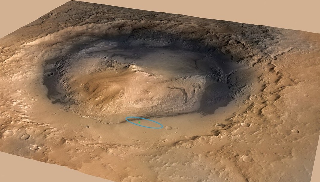
Gale crater, about the size of Connecticut and Rhode Island together, with Mount Sharp in its middle; the green dot inside the blue ellipse is where Curiosity landed. NASA/JPL-Caltech/ESA/DLR/FU Berlin/MSSS, PIA16058.

An engineer fits one of the REMS booms to Curiosity's mast in 2011. NASA/JPL-Caltech, via Wikimedia Commons.

6. What earlier studies found.
- Haberle and others (2014) read REMS's first 100 sols. The sensor worked well and showed the CO2 cycle, and daily pressure swings (the "thermal tides") several times larger than other landers had seen, partly because the crater amplifies them. doi:10.1002/2013JE004488
- Guzewich and others (2019) describe the 2018 global dust storm from Curiosity: the dust hid 97% of the Sun's ultraviolet light at the ground, the day-to-night temperature range fell by 30 K, and the pressure wave that rises and falls twice a day grew to an amplitude of 40 Pa. doi:10.1029/2018GL080839
- Lange and others (2022) compared the pressure measured by two landers 40 years apart, Viking 1 and InSight: the CO2 cycle changed by no more than 8 Pa. They saw hints of a larger north polar cap after the 2018 storm, with no agreed cause. doi:10.1029/2022JE007190
- de la Torre Juárez and others (2024) compared the Gale record before and after the 2018 storm and found the pressure lower than usual after it, a deficit later dust storms did not erase, and, from an orbiter, a larger north polar cap. doi:10.1029/2023JE007810
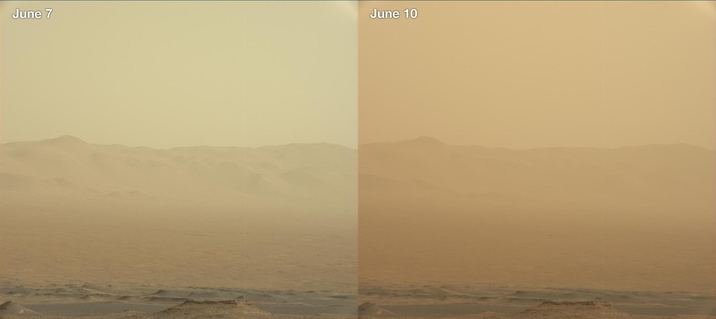
The same view of Gale crater's rim from Curiosity on 7 and 10 June 2018: in three days the global dust storm hid it. NASA/JPL-Caltech/MSSS, PIA22520.
7. What is still open, and what you will do. Whether the 2018 storm really changed how much air Mars holds, and why, is still argued: a dusty crater, a bigger polar cap or a sensor are all on the table. You will build the model one part at a time: show that the 6% drop is the climb, measure from the readings how fast air thins with height, forecast a Mars year the model has not seen, find the storm's mark in what the model misses, and enter a forecast for Mars year 38 on the leaderboard.
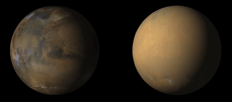
Mars from the Mars Reconnaissance Orbiter in May 2018 (left) and July 2018 (right), when dust covered the whole planet. NASA/JPL-Caltech/MSSS, PIA22487.
How this notebook works
This notebook is built like a weekly notebook: a few questions lead it, each section answers one, and every place you work opens with a pencil icon ✏️ and the words Your turn. The difference is how much you write. Each Your turn says why the step matters and gives a numbered plan in words; the cell under it is empty, and you write all of the code, looking back at the weekly notebook it names. A self-check cell follows. Run it: it tells you whether your numbers are right, as in every week.
The last Your turn is your leaderboard entry: it saves the file submission.csv. Run every cell so your answers and figures are saved in the file, then download this notebook itself — the .ipynb file — and upload it to Gradescope together with submission.csv. In JupyterLab: File ▸ Download, or right-click the file in the left-hand panel and choose Download. The leaderboard scores your file on answers you never see and ranks everyone's entries.
Two habits from the first minute. A cell runs when you press Shift+Enter, and the notebook remembers everything it has already run — so when something breaks and you cannot see why, Kernel → Restart Kernel and Run All Cells throws the memory away and rebuilds it from the top. That is never the wrong thing to do.
What you'll be able to do
The science. Say why the air pressure on Mars rises and falls twice every year, why a rover that climbs a mountain measures less air, how the height over which air thins (the scale height) follows from the temperature, and what a planet-wide dust storm did to the air.
The code. You write every line: a plot with a loop over the years, a function for the typical
miss, a function that makes seasonal columns, LinearRegression on the log of the pressure, a
mean for each group, a split by Mars year, a choice made on a held-out year, a bootstrap over
blocks of sols, a paired bootstrap of two models, and a submission.csv file.
The four questions of the project:
- How does the air pressure change through a Mars year, and from year to year?
- Can the seasons alone predict the pressure, or does the rover's climb matter?
- How well does the model forecast a Mars year it has never seen?
- Did the 2018 dust storm leave a mark, and is the forecast better without it?
What you hand in, and when
One Gradescope assignment, "Final project: Mars weather", takes everything.
- Individual work. Start now; Gradescope takes uploads from Wed 25 Nov, and the project is due Wed 16 Dec. Mon 7 Dec (RRR week) has no class, but you are welcome to come to the room in class time and work on your notebook.
- Every upload carries two files:
submission.csv(your leaderboard entry, made by the last Your turn) and this notebook. Gradescope cannot check this for you, so follow these steps:- In DataHub, save the notebook (File ▸ Save).
submission.csvis in the same folder as the notebook, in the left-hand panel. - Download both: right-click each file in the left-hand panel and choose Download.
- In Gradescope, open Final project: Mars weather, click Upload Submission, and select both files (hold Ctrl, or Cmd on a Mac, to select the second), or drag both into the window. Type a name for the leaderboard: your own name or a nickname. Your classmates will see it next to your score.
- Check that Gradescope lists both files, then upload. If the result says a file is missing, upload both again.
- In DataHub, save the notebook (File ▸ Save).
- Up to 10 uploads that change
submission.csvare scored on the leaderboard. An upload that changes only the notebook is free. - Everything is due Wed 16 Dec at 23:59 Pacific time: the notebook and your last entry.
- Before every upload: Kernel → Restart Kernel and Run All Cells must run from top to bottom without an error.
How it is graded (100 points). The Your turns are graded like a week's. The leaderboard gives two grades: one for a valid entry that beats the same season one year earlier, and one for your rank, on the final score from the hidden part of the board. Choose your entry by your own fair test, not by the public score.
| What | Points | Graded by | Full marks when |
|---|---|---|---|
| Your turns 1 to 12 | 80 | Gradescope, when you upload | each Your turn by its self-check (Your turn 1, a figure, for being done and run), and the notebook runs from top to bottom without an error |
| Leaderboard entry | 10 | Gradescope, pass or fail | your last submission.csv is valid and its final score beats guessing each sol from the same season of Mars year 37 |
| Leaderboard rank | 10 | after the board closes | your final score, on the hidden part, ranked among the students on this project: top quarter 10, second quarter 8, third quarter 6, last quarter 4; a tie takes the higher band; no valid entry 0 |
Setup
Run the next two cells once. All their code is given. Three files ship with the course:
trackT13_mars_daily.csv: the sols from the landing, in Mars year 31, to the end of Mars year 37, your training file;trackT13_mars_year38_inputs.csv: the leaderboard file, 608 sols of Mars year 38, from its start to Ls 341, with the season and the rover's height but not the pressure;trackT13_submission_template.csv: the empty submission template, one row per leaderboard sol.
import numpy as np
from sklearn.linear_model import LinearRegression
import pandas as pd
import matplotlib.pyplot as plt

# house style, set once, so every plot cell below holds only what matters
plt.rcParams.update({"figure.figsize": (7, 4.5), "figure.dpi": 110,
                     "axes.grid": True, "grid.alpha": 0.3, "axes.axisbelow": True})

CACHE = "https://raw.githubusercontent.com/AI4EPS/EPS88_PyEarth/main/data"

mars = pd.read_csv(CACHE + "/trackT13_mars_daily.csv")
leaderboard = pd.read_csv(CACHE + "/trackT13_mars_year38_inputs.csv")
template = pd.read_csv(CACHE + "/trackT13_submission_template.csv")
print("training file, as it arrives:", mars.shape)
print("leaderboard file:", leaderboard.shape)

# larger lettering for this project's figures
plt.rcParams.update({"font.size": 11, "axes.titlesize": 12, "legend.fontsize": 9})
The next cell keeps the sols with a pressure. Its columns: sol, counted from the landing;
terrestrial_date, the date on Earth; ls, the season (section 1 explains it); mars_year;
pressure in pascals (Pa); the lowest and highest air temperature of the sol, min_temp and
max_temp, in °C; and elev_m, the rover's height in metres above the areoid, Mars's "sea
level" (a level surface drawn around the planet, since Mars has no sea); Gale crater lies below it,
so the heights are negative. The leaderboard file has no temperatures, so a model for it can
use only ls and elev_m.
train = mars[mars["pressure"].notna()].reset_index(drop=True)

print("sols with a pressure:", len(train), "  without:", mars["pressure"].isna().sum())
print("Mars years:", train["mars_year"].min(), "to", train["mars_year"].max())
print("dates:", train["terrestrial_date"].min(), "to", train["terrestrial_date"].max())
print(train.head())
1. How does the air pressure change through a Mars year, and from year to year?
The season is counted by ls, Mars's position around the Sun, in degrees. Ls = 0 is the start
of northern spring, 90 of northern summer, 180 of northern autumn and 270 of northern winter. One
full circle, a Mars year, takes 668 sols; Mars year 32 began on
2013-08-01 on Earth. Curiosity sits in Gale crater, a little south of the equator.
Does the record sink from year to year? The next cell draws every reading against time, and marks the highest reading of each Mars year with its value.
plt.figure(figsize=(10, 4.5))
plt.plot(train["sol"], train["pressure"], ".", markersize=2, color="0.5")
for year in range(31, 38):
    one_year = train[train["mars_year"] == year]
    top = one_year.iloc[np.argmax(one_year["pressure"])]     # the year's highest reading
    plt.plot(top["sol"], top["pressure"], "v", color="tab:red", markersize=8)
    plt.text(top["sol"], top["pressure"] + 8, f"{top['pressure']:.0f}", ha="center", color="tab:red")
    plt.text(np.mean(one_year["sol"]), 665, f"year {year}", ha="center", fontsize=9)
    plt.axvline(np.min(one_year["sol"]), color="0.8", lw=1)  # where each Mars year starts
plt.ylim(655, 950)
plt.xlabel("sol (Mars days since landing)")
plt.ylabel("pressure (Pa)")
plt.title(f"Air pressure at Curiosity, {len(train)} sols: each year's highest reading in red")
plt.show()
The pressure goes up and down every Mars year, and the whole pattern sinks. The highest reading of Mars year 32 was 925 Pa; that of Mars year 37, 871 Pa. To see whether the shape of the year is the same each time, put every year on the same season axis.
✏️ Your turn 1
Does the pressure follow the same seasonal shape every Mars year?
Why: before any model, look at the data. If each year has the same shape, a model of the season should work; if the years differ, something else is changing.
Look back at: the loop that drew several curves with a legend, from When will CO2 pass 450
ppm? (07_co2_450_ppm.ipynb).
- Loop over the Mars years 31 to 37. For each one, take its rows of
trainand plotpressure(up) againstls(across), as small dots or a thin line, labelled with the year. - Label both axes with their units, add a legend, and give the plot a title.
This Your turn has no self-check: a figure you can see needs none. A good figure shows seven
curves you can tell apart, each rising and falling twice between Ls 0 and 360, with the years in
order in the legend. Colours that run in order from the first year to the last (for example
color=plt.cm.viridis((year - 31) / 6)) make it easy to see whether the later years sit lower.
# ← your answer here: write your code here
Every year has the same shape, two highs and two lows, and every curve sits below the one before. Near Ls 256, the highest point of the year, Mars year 32 averaged 917 Pa and Mars year 37 859 Pa. The two lows are the two winters, when one polar cap is taking air out of the sky: the deep low near Ls 153 is southern winter, the shallower one near Ls 342 northern winter.
Think. If the drop from year to year is real, Mars is losing its air fast. Is it?
✏️ Your turn 2
How far off is the simplest guess: the same pressure for every sol?
Why: every model in this notebook has to beat the number you find here.
Baseline: Write the dumbest rule you can, first. Any model that cannot beat it is decoration.
Typical miss: Square every gap between what happened and what the curve said, average the squares, and take the square root: the usual size of a miss, in the data's own units.
Look back at: the typical miss, from When will CO2 pass 450 ppm? (07_co2_450_ppm.ipynb).
- Write a function
typical_miss(errors)that takes a column of errors and returns their typical miss. You will use it for every model in this notebook. - The rule: guess the average
pressureof all the training sols. Name itaverage_pressure. - Each sol's error is its
pressureminus that guess. Their typical miss isbaseline_miss. - Print the guess and the typical miss, in Pa.
Use these names, because the self-check looks for them: typical_miss, average_pressure,
baseline_miss.
# ← your answer here: write your code here
# the self-check reads: typical_miss, average_pressure, baseline_miss
# Self-check: run this after your answer. You do not need to read it — it only says whether something is off.
assert abs(typical_miss(np.array([3.0, -4.0])) - np.sqrt(12.5)) < 1e-9, \
    "the typical miss of the errors 3 and -4 is the square root of (9 + 16) / 2"
assert abs(average_pressure - 822.369) < 0.01, \
    "the guess is the average pressure of the training sols"
assert abs(baseline_miss - 56.698) < 0.01, \
    "the typical miss of each sol's pressure minus that average"
print(f"✓ Your turn 2 — always guessing {average_pressure:.1f} Pa misses by {baseline_miss:.1f} Pa")
Always guessing 822 Pa misses by 56.7 Pa. That is the bar: a model that cannot beat 56.7 Pa has learned nothing from the season.
2. Can the seasons alone predict the pressure, or does the rover's climb matter?
Mars's pressure needs more than the one wave a year that CO2 on Earth needed. In the CO2 week a pair of seasonal columns did the job:
Seasonal column: A column that rises and falls once a year, so the fitted curve can rise and fall with the seasons.
One pair, the sine and the cosine of the month's angle, was enough there, because CO2 rises and falls once a year. Mars's pressure rises and falls twice, with highs of different heights, and one pair can draw only one high.
More pairs draw more shapes. A second pair goes round twice a year, a third three times. With
the angle of the season in radians, $\theta$ = np.radians(ls), the pairs are
$$\sin\theta,\ \cos\theta,\quad \sin 2\theta,\ \cos 2\theta,\quad \sin 3\theta,\ \cos 3\theta,\ \dots$$
and linear regression finds how much of each to add:
$$p = a + b_1 \sin\theta + c_1 \cos\theta + b_2 \sin 2\theta + c_2 \cos 2\theta + \dots$$
Linear regression: Draw the best straight line. Best means the smallest root mean squared error: the line that misses its points least.
With many columns it finds the best mix of all of them in the same way. The next cell draws the sine of each of the first three pairs.
ls_values = np.arange(0, 361)
plt.figure(figsize=(9, 3.8))
for n in [1, 2, 3]:
    plt.plot(ls_values, np.sin(np.radians(n * ls_values)), lw=2, label=f"pair {n}: the sine of {n} × the angle")
plt.axhline(0, color="k", lw=0.8)
plt.xticks([0, 90, 180, 270, 360])
plt.xlabel("season, Ls (degrees)")
plt.ylabel("value of the column")
plt.title("The building blocks: waves that go round 1, 2 and 3 times a Mars year")
plt.legend(loc="upper center", bbox_to_anchor=(0.5, -0.22), ncol=3)
plt.show()
✏️ Your turn 3
How close do three seasonal pairs get?
Why: if the seasons were all there is, this model would follow every year.
Look back at: functions and LinearRegression, from How old is the universe?
(06_age_of_the_universe.ipynb), and the seasonal columns of the CO2 week.
- Write a function
add_season_columns(table, n_pairs). It adds totableone sine and one cosine column for each n from 1 ton_pairs, of n times the angle oflsin radians, and returns the list of the names it added. Name the columns as you like. season_columns: what your function returns fortrainwith 3 pairs.- Fit a
LinearRegressionofpressureon those six columns, for every training sol. Name itseason_fit, and add its prediction as the columnseasonoftrain. season_miss: its typical miss, in Pa. Print it besidebaseline_miss.
Use these names, because the self-check looks for them: add_season_columns,
season_columns, season_fit, season_miss.
# ← your answer here: write your code here
# the self-check reads: add_season_columns, season_columns, season_fit, season_miss
# Self-check: run this after your answer. You do not need to read it — it only says whether something is off.
probe = pd.DataFrame({"ls": np.arange(0, 360, 5)})
probe_columns = add_season_columns(probe, 2)
angle = np.radians(probe["ls"])
shape = 2 * np.sin(2 * angle) - np.cos(angle) + 0.5 * np.cos(2 * angle)   # needs both pairs
probe_fit = LinearRegression().fit(probe[probe_columns], shape)
assert len(probe_columns) == 4 and probe_fit.score(probe[probe_columns], shape) > 0.9999, \
    "add_season_columns(table, 2) should add and return four columns: the sine and cosine of the angle and of twice the angle"
assert len(season_columns) == 6, "season_columns: the six column names for three pairs"
assert abs(season_miss - 19.415) < 0.05, \
    "fit pressure on the six seasonal columns of every training sol; the typical miss of pressure minus the prediction"
print(f"✓ Your turn 3 — three seasonal pairs miss by {season_miss:.1f} Pa, always the average by {baseline_miss:.1f} Pa")
The fitted season beside the data. The next cell draws the season curve over the readings of the first and the last full year.
# season_fit and season_columns: Your turn 3
ls_table = pd.DataFrame({"ls": np.arange(0, 360)})
add_season_columns(ls_table, 3)
season_curve = season_fit.predict(ls_table[season_columns])    # the fitted pressure at each whole Ls
plt.figure(figsize=(9, 5))
plt.plot(train["ls"], train["pressure"], ".", markersize=1, color="0.85", label="all seven years")
for year, colour in [(32, "tab:blue"), (37, "tab:red")]:
    one_year = train[train["mars_year"] == year]
    plt.plot(one_year["ls"], one_year["pressure"], ".", markersize=3, color=colour, label=f"Mars year {year}")
plt.plot(ls_table["ls"], season_curve, color="k", lw=2.5, label="the fitted season (three pairs)")
plt.annotate("Mars year 32 sits above the curve", xy=(60, 900), xytext=(80, 935), arrowprops={"arrowstyle": "->"})
plt.annotate("Mars year 37 sits below it", xy=(300, 797), xytext=(250, 730), arrowprops={"arrowstyle": "->"})
plt.ylim(680, 950)
plt.xlabel("season, Ls (degrees)")
plt.ylabel("pressure (Pa)")
plt.title(f"One season curve for all seven years: typical miss {season_miss:.1f} Pa")
plt.legend(loc="lower left")
plt.show()
The curve has the right shape but one height for every year: too low for Mars year 32 and too high for Mars year 37. It misses by 19.4 Pa, against 56.7 Pa for always the average. Does it miss each year in its own way?
Residual: A residual is the real value minus the line's value.
Here a sol's residual is its pressure minus the model's
prediction: above zero, the air pressed harder than the model said.
✏️ Your turn 4
Does the seasonal model miss every Mars year in the same way?
Why: a good model's residuals average zero in every year. A steady fall from year to year means something the season columns do not hold is changing.
Look back at: groupby, from Earth's elevation has two peaks (03_two_peaks.ipynb).
- Add the column
season_residualtotrain:pressureminus the seasonal prediction. season_by_year: its mean in each Mars year. Print it, rounded to 1 place.- Plot it: one bar per Mars year (
plt.bar), the mean residual up, with a horizontal line at zero. Label both axes and give a title. A good figure shows at a glance which years sit above zero and which below; writing each bar's value on it (plt.text) makes the trend readable without the printout.
Use these names, because the self-check looks for them: season_by_year.
# ← your answer here: write your code here
# the self-check reads: season_by_year
# Self-check: run this after your answer. You do not need to read it — it only says whether something is off.
assert len(season_by_year) == 7, "season_by_year: one mean residual for each of the Mars years 31 to 37"
assert abs(season_by_year[37] - (-30.199)) < 0.1, \
    "the mean, over the sols of each Mars year, of pressure minus the seasonal prediction"
print(f"✓ Your turn 4 — Mars year 32 sits {season_by_year[32]:+.1f} Pa from the season curve, Mars year 37 {season_by_year[37]:+.1f} Pa")
The residual falls every year, from +22.7 Pa in Mars year 32 to -30.2 Pa in Mars year 37. Read alone, that says Mars lost a few percent of its air in a few years. But the barometer was not standing still. The next cell draws the rover's height on each sol.
lowest = train.iloc[np.argmin(train["elev_m"])]      # the sol on which the rover stood lowest
highest = train.iloc[np.argmax(train["elev_m"])]     # and highest
climb = highest["elev_m"] - lowest["elev_m"]
plt.figure(figsize=(10, 4))
plt.plot(train["sol"], train["elev_m"], color="tab:brown", lw=2)
for year in range(31, 38):
    one_year = train[train["mars_year"] == year]
    plt.axvline(np.min(one_year["sol"]), color="0.8", lw=1)
    plt.text(np.mean(one_year["sol"]), -3650, f"year {year}", ha="center", fontsize=9)
plt.annotate(f"lowest, near the landing site: {lowest['elev_m']:,.0f} m", xy=(lowest["sol"], lowest["elev_m"]),
             xytext=(1900, -4480), arrowprops={"arrowstyle": "->"})
plt.annotate(f"highest: {highest['elev_m']:,.0f} m, {climb:,.0f} m above the lowest",
             xy=(highest["sol"], highest["elev_m"]), xytext=(1700, -3760), arrowprops={"arrowstyle": "->"})
plt.ylim(-4600, -3600)
plt.xlabel("sol (Mars days since landing)")
plt.ylabel("rover height (m)")
plt.title("Curiosity's climb up Mount Sharp, Mars years 31 to 37")
plt.show()
# season_residual: Your turn 4; the residual against the rover's height, with a straight line
line_fit = LinearRegression().fit(train[["elev_m"]], train["season_residual"])
per_100_m = line_fit.coef_[0] * 100                   # Pa of residual for each 100 m of climb
heights = pd.DataFrame({"elev_m": [np.min(train["elev_m"]), np.max(train["elev_m"])]})

plt.figure(figsize=(8, 5))
plt.scatter(train["elev_m"], train["season_residual"], s=3, c=train["mars_year"], cmap="viridis")
plt.colorbar(label="Mars year")
plt.plot(heights["elev_m"], line_fit.predict(heights), color="tab:red", lw=2.5,
         label=f"straight line: {per_100_m:.1f} Pa per 100 m of climb")
plt.axhline(0, color="k", lw=0.8)
plt.xlabel("rover height (m)")
plt.ylabel("residual of the seasons alone (Pa)")
plt.title(f"What the season misses, against height, {len(train)} sols")
plt.legend(loc="upper right")
plt.show()
Curiosity climbed 848 m, from -4,521 m to -3,673 m, and the higher it stood, the lower the residual: about 7.4 Pa less for every 100 m. On a mountain there is less air above you, so it presses less: the year-to-year fall is the climb, not the planet.
Air pressure falls with height in a known way. Each metre up takes away the weight of one metre of air, and the thinner the air, the less a metre of it weighs. So the pressure falls by the same fraction with every metre:
$$p = p_0\, e^{-z/H} \qquad\text{so}\qquad \ln p = \ln p_0 - \frac{z}{H}$$
- $p$ is the pressure and $z$ the height,
elev_m; - $p_0$ is the pressure at height 0, which changes with the season;
- $H$ is the scale height: the climb over which the pressure falls by a factor of e, about 2.7.
In logs, the height is one more straight-line column. So fit np.log(pressure) on the seasonal
columns and elev_m: the seasonal columns give $\ln p_0$, the coefficient of elev_m is
$-1/H$, and np.exp turns a prediction back into pascals.
✏️ Your turn 5
With the rover's height added, how small is the miss, and what scale height does the fit find?
Why: if the climb explains the fall from year to year, adding it should shrink the miss many times over, and the fitted $H$ should agree with the physics of the air.
Look back at: your Your turn 3, and np.log and np.exp.
height_columns: your three-pairseason_columnspluselev_m.- Fit a
LinearRegressionof the natural log ofpressureon them, for every training sol. Name itheight_fit. - Add its prediction, turned back into Pa, as the column
height_modeloftrain. height_miss: its typical miss in Pa. Print it besideseason_miss.H_km: the scale height in km, from the coefficient ofelev_m, which is $-1/H$ with $H$ in metres. Print it.
Use these names, because the self-check looks for them: height_fit, height_miss, H_km.
# ← your answer here: write your code here
# the self-check reads: height_fit, height_miss, H_km
# Self-check: run this after your answer. You do not need to read it — it only says whether something is off.
assert height_miss < season_miss / 3, \
    "with the height the miss should fall many times: fit the LOG of pressure, and turn the prediction back with np.exp"
assert abs(height_miss - 3.739) < 0.05, \
    "fit ln pressure on the three seasonal pairs and elev_m, for every training sol; the typical miss in Pa"
assert 9 < H_km < 13, "H_km: minus one over the coefficient of elev_m, turned from metres into km"
print(f"✓ Your turn 5 — with the height the miss is {height_miss:.2f} Pa; scale height {H_km:.1f} km")
Physics gives the scale height too: $H = RT/(mg)$, where $T$ is the air temperature in kelvin, $R$ the gas constant, $m$ the mass of one mole of the air and $g$ the pull of gravity. Warmer air spreads higher; stronger gravity pulls it lower. The next cell computes it from the air temperatures REMS measured.
# H_km: Your turn 5
R = 8.314          # gas constant, J per mol per kelvin
m_co2 = 0.04401    # kg per mol of carbon dioxide; Mars's air is about 95% CO2
g_mars = 3.71      # m/s², the pull of gravity at Mars's surface (NASA Mars fact sheet)

T_air = np.mean((train["min_temp"] + train["max_temp"]) / 2) + 273.15   # °C to kelvin
H_physics_km = R * T_air / (m_co2 * g_mars) / 1000
print("mean air temperature:", round(T_air), "K   scale height from physics:", round(H_physics_km, 1), "km")
print("scale height from your fit (Your turn 5):", round(H_km, 1), "km")
The fit's scale height, 11.0 km, is within a kilometre of the physics, 11.7 km at 230 K. Nothing told the regression about gas, gravity or temperature, and it found the thinning of air with height from the rover's readings. With the height added the miss falls from 19.4 Pa to 3.74 Pa. Mars is not losing its air; Curiosity is climbing.
But 3.74 Pa is a score on the sols the model was fitted to. The leaderboard asks about a year the model has never seen, so the next section asks the same.
3. How well does the model forecast a Mars year it has never seen?
A model is judged on data it did not learn from.
Train/test split: Hide some data from yourself, then check.
But which sols to hide? Not sols picked at random. The weather of one sol is much like that of the sol before and after, so a model that has seen sol 2,000 and sol 2,002 has nearly seen sol 2,001, and the test would be too kind. And the leaderboard does not hide scattered sols: it hides most of a Mars year, 38 up to Ls 341, at heights the rover had not reached. So we split by structure, the way the leaderboard does, one year earlier: fit on Mars years 31 to 36, and hide Mars year 37.
A fair baseline for a new year is not the average of all sols, which ignores the season, but
the same season one year earlier: for each sol of Mars year 37, the pressure
Curiosity read at the same ls in Mars year 36. It is the leaderboard's pass line.
✏️ Your turn 6
How far off is "the same season last year" on a Mars year it has not seen?
Why: this is the bar a forecast of a new year must clear, and the leaderboard's pass line.
Look back at: the split by time, from When will CO2 pass 450 ppm? (07_co2_450_ppm.ipynb),
and groupby.
fit_part: the rows oftrainfrom Mars years 31 to 36.hidden_part: the rows of Mars year 37. Take a.copy()of each, because you will add columns. Print how many sols each holds.- From
fit_part, the mean pressure of Mars year 36 at each value ofls. - For each hidden sol, that mean at its own
ls. A few values oflshave no sol in Mars year 36; leave those sols out of the score (.dropna()drops them). last_year_miss: the typical miss of the hidden pressure minus that guess. Print it, and the mean of the errors: is the guess too high or too low?
Use these names, because the self-check looks for them: fit_part, hidden_part,
last_year_miss.
# ← your answer here: write your code here
# the self-check reads: fit_part, hidden_part, last_year_miss
# Self-check: run this after your answer. You do not need to read it — it only says whether something is off.
assert len(hidden_part) == 633 and set(hidden_part["mars_year"]) == {37}, \
    "the hidden part is every sol of Mars year 37"
assert len(fit_part) + len(hidden_part) == len(train), "every sol is in exactly one part"
assert abs(last_year_miss - 15.864) < 0.3, \
    "for each hidden sol, the Mars year 36 pressure at the same ls; the typical miss of the hidden pressure minus it"
print(f"✓ Your turn 6 — the same season last year misses Mars year 37 by {last_year_miss:.2f} Pa")
The same season last year misses by 15.86 Pa, and almost all of it is one way: on average it guesses 15.1 Pa too high. Over Mars year 37 the rover climbed another 190 m, and last year's readings were taken lower down. Your model knows the height. How many seasonal pairs should it use?
Three was a guess. Too few pairs and the season's shape leaks into the height column; too many and the curve starts to follow the noise of the years it was fitted to. So the number of pairs is chosen on the hidden year:
Validation years: Years held back to choose between models. Once they have chosen, they are no longer a fair test.
Here, as in the CO2 week, the hidden year does both jobs: it chooses the number of pairs, and then it scores the choice, so that score is a little kind. Section 4 comes back to this.
When two numbers of pairs miss by almost the same amount, take the fewer. A difference of a hundredth of a pascal is far smaller than how much the score would move with another year, and fewer columns are fewer things the fit can get wrong at heights it has not seen.
✏️ Your turn 7
How many seasonal pairs forecast the hidden year best?
Why: the number of pairs is a choice, and a choice is made on data the fit has not seen.
Look back at: choosing between curves on held-back years, from When will CO2 pass 450 ppm?
(07_co2_450_ppm.ipynb), and your Your turns 3 and 5.
- For each number of pairs from 1 to 8: add that many pairs to
fit_partand tohidden_partwith youradd_season_columns; fit the log ofpressureon them andelev_m, onfit_partonly; predict the hidden sols, back in Pa; and find the typical miss. miss_by_pairs: those misses, keyed by the number of pairs (a dict or a Series). Print it.chosen_pairs: the fewest pairs whose miss is within 0.01 Pa of the smallest miss.test_miss: its miss. Print both besidelast_year_miss.- Plot the miss (up) against the number of pairs (across), with a horizontal line at
last_year_miss. A log scale on the miss axis (plt.yscale("log")) shows the small and the large misses together. A good figure also marks the chosen number of pairs, so a reader sees at once which point won and by how much it beats last year's guess.
Use these names, because the self-check looks for them: miss_by_pairs, chosen_pairs,
test_miss.
# ← your answer here: write your code here
# the self-check reads: miss_by_pairs, chosen_pairs, test_miss
# Self-check: run this after your answer. You do not need to read it — it only says whether something is off.
tried = pd.Series(miss_by_pairs, dtype=float)
assert len(tried) >= 6 and 1 in tried.index, "miss_by_pairs: the hidden miss for each number of pairs from 1 to 8"
ties = [n for n in tried.index if tried[n] <= tried.min() + 0.01]   # within 0.01 Pa of the best
assert chosen_pairs == min(ties), \
    "chosen_pairs: the FEWEST pairs whose miss on the hidden year is within 0.01 Pa of the smallest"
assert abs(test_miss - tried[chosen_pairs]) < 1e-6, "test_miss: the miss at chosen_pairs"
check_fit, check_hidden = fit_part.copy(), hidden_part.copy()
check_columns = add_season_columns(check_fit, chosen_pairs) + ["elev_m"]
add_season_columns(check_hidden, chosen_pairs)
check_model = LinearRegression().fit(check_fit[check_columns], np.log(check_fit["pressure"]))
check_miss = typical_miss(check_hidden["pressure"] - np.exp(check_model.predict(check_hidden[check_columns])))
assert abs(test_miss - check_miss) < 0.02, \
    "fit ln pressure on the pairs and elev_m of fit_part only; the typical miss in Pa of the hidden pressure minus np.exp of the prediction"
assert tried[1] > 4 * test_miss, "one pair alone should miss the hidden year badly"
print(f"✓ Your turn 7 — {chosen_pairs} pairs: {test_miss:.2f} Pa on the hidden year; one pair {tried[1]:.1f} Pa; same season last year {last_year_miss:.2f} Pa")
4 pairs miss the hidden year by 3.85 Pa, a quarter of the 15.86 Pa of the same season last year. 4 and 5 pairs tie: their misses differ by less than 0.01 Pa, so the rule takes the fewer. One pair misses by 39.1 Pa, worse than last year's guess: with one wave the fit cannot draw Mars's two highs, so it pushes the misfit into the height column, and a wrong height column forecasts a higher rover badly. Three pairs miss by 4.57 Pa; from four pairs on the miss barely moves (3.87 Pa with eight).
3.85 Pa is one hidden year. A different year would give a slightly different miss. How different?
Bootstrap: Ask the data the same question a thousand times, using a different random slice of itself each time.
The slice cannot be single sols, for the same reason the split could not: neighbouring sols miss together. So we cut the hidden year into blocks of 30 sols, about a month, and redraw whole blocks, as the leaderboard does for its own interval. A redraw's typical miss is the square root of (all the squared errors its blocks hold ÷ all the sols they hold), as in the week of the bootstrap.
✏️ Your turn 8
How much could the hidden-year score move with other months like these?
Why: two models whose scores differ by less than this are not clearly different. You will need it in the next section.
Look back at: the bootstrap, from How long was the Earth frozen? (08_how_long_frozen.ipynb).
- Fit the chosen model again on
fit_part(chosen_pairspairs andelev_m, the log ofpressure). Name itchosen_fit, and add its prediction for each hidden sol, in Pa, as the columnwith_stormofhidden_part. (The next section explains the name.) Its typical miss, with yourtypical_miss, should be yourtest_miss. - Number each hidden sol's block: its
solminus the first hidden sol, divided by 30 and rounded down (//). per_block: one row per block, with the sum of its squared errors and its number of sols.- Make a random generator,
rng = np.random.default_rng(88), and an empty list,redrawn_misses. 1,000 times: redraw as many blocks asper_blockholds, with replacement (random_state=rng), and append the redraw's typical miss. test_interval: the 2.5th and 97.5th percentiles of the 1,000 misses. Print it besidetest_miss.- Draw a histogram of the 1,000 misses, with vertical lines at the two ends of the interval and
at
test_miss.
Use these names, because the self-check looks for them: chosen_fit, per_block,
redrawn_misses, test_interval.
# ← your answer here: write your code here
# the self-check reads: chosen_fit, per_block, redrawn_misses, test_interval
# Self-check: run this after your answer. You do not need to read it — it only says whether something is off.
assert abs(typical_miss(hidden_part["pressure"] - hidden_part["with_storm"]) - test_miss) < 0.02, \
    "with_storm: the chosen model's prediction in Pa for each hidden sol, fitted on fit_part"
assert 15 <= len(per_block) <= 30 and per_block.sum().max() >= len(hidden_part), \
    "per_block: one row per 30-sol block, with the sum of the squared errors and the number of sols"
assert len(redrawn_misses) == 1000 and abs(np.mean(redrawn_misses) - test_miss) < 0.3, \
    "1,000 redraws, each the square root of the redrawn squared errors over the redrawn sols"
assert test_interval[0] < test_miss < test_interval[1] and 0.3 < test_interval[1] - test_interval[0] < 4, \
    "test_interval: the 2.5th and 97.5th percentiles of the 1,000 redrawn misses"
print(f"✓ Your turn 8 — 95% interval {test_interval[0]:.2f} to {test_interval[1]:.2f} Pa around {test_miss:.2f}")
The forecast beside the year it never saw. The next cell draws Mars year 37's readings with your model's forecast and with the guess "same season last year".
# hidden_part: Your turns 6 and 8; with_storm is the chosen model's forecast
# the old guess again: Mars year 36's mean pressure at each whole Ls, looked up for each hidden sol
same_season = fit_part[fit_part["mars_year"] == 36].groupby("ls")["pressure"].mean()
same_season_guess = hidden_part["ls"].map(same_season)
plt.figure(figsize=(10, 4.5))
plt.plot(hidden_part["sol"], hidden_part["pressure"], ".", markersize=4, color="0.4", label="what Curiosity read")
plt.plot(hidden_part["sol"], same_season_guess, color="tab:red", lw=1.5, ls="--",
         label=f"same season last year: misses by {last_year_miss:.1f} Pa")
plt.plot(hidden_part["sol"], hidden_part["with_storm"], color="tab:purple", lw=2,
         label=f"your model ({chosen_pairs} pairs and height): misses by {test_miss:.2f} Pa")
plt.xlabel("sol (Mars days since landing)")
plt.ylabel("pressure (Pa)")
plt.title(f"Forecasts of Mars year 37, {len(hidden_part)} sols the model never saw")
plt.legend(loc="upper center", bbox_to_anchor=(0.5, -0.15))
plt.show()
Last year's guess runs above the readings almost all year; the model, which knows the rover climbed, follows them. The forecast of the hidden year misses by 3.85 Pa, with a 95% interval from 3.01 to 4.62 Pa. The interval is 1.6 Pa wide, because 23 blocks is not many: one bad month moves the score.
4. Did the 2018 dust storm leave a mark, and is the forecast better without it?
The global dust storm of the Background (step 6) began in early June 2018; the file reaches Ls 185 of Mars year 34 on 2018-05-31, sol 2068. Dust in the air soaks up sunlight and warms the air, which changes the winds and how much carbon dioxide freezes onto the polar caps. De la Torre Juárez and others (2024) found the pressure at Gale about 3 to 6 Pa lower than usual after the storm. If the storm left a mark, your model's residuals should show it, and a model fitted on a year the storm disturbed may have learned the wrong season.
✏️ Your turn 9
After the storm began, did the air press less than the model says?
Why: a mark the storm left is a residual: a few pascals below zero, starting when it began.
Look back at: your Your turns 4 and 8.
- Add the column
residualtofit_part:pressureminus the prediction ofchosen_fit(Your turn 8) for every fitting sol, in Pa. storm_residual: the mean residual over the sols of Mars year 34 from Ls 185 on, the storm and the half year after it.calm_residual: the mean residual over the sols of Mars years 32 and 33 from Ls 185 on: the same season in two years with no global storm. Print both.- Plot the residual (up) against
sol(across) as small dots, with a horizontal line at zero and a vertical line at the first sol of Mars year 34 from Ls 185 on. A good figure makes a dip of a few pascals visible: limit the vertical axis to about ±12 Pa (plt.ylim), and draw the mean residual of each 30-sol stretch as a line on top of the dots (agroupby, as for the blocks of Your turn 8).
Use these names, because the self-check looks for them: storm_residual, calm_residual.
# ← your answer here: write your code here
# the self-check reads: storm_residual, calm_residual
# Self-check: run this after your answer. You do not need to read it — it only says whether something is off.
assert "residual" in fit_part and abs(np.mean(fit_part["residual"])) < 1, \
    "fit_part's residual column: pressure minus the chosen model's prediction in Pa"
storm_sols_34 = fit_part[(fit_part["mars_year"] == 34) & (fit_part["ls"] >= 185)]
assert abs(storm_residual - np.mean(storm_sols_34["residual"])) < 0.01, \
    "storm_residual: the mean residual over Mars year 34 from Ls 185 on"
assert -6 < storm_residual < -2 and -1.5 < calm_residual < 1.5, \
    "check the signs: a residual is pressure minus the prediction; calm_residual is Mars years 32 and 33 from Ls 185 on"
print(f"✓ Your turn 9 — after the storm {storm_residual:+.2f} Pa, the same season in calm years {calm_residual:+.2f} Pa")
From the storm on, Mars year 34 sits 3.5 Pa below the model, where the same season of Mars years 32 and 33 sits +0.3 Pa from it. That is the size the 2024 study found, from one rover and a model you wrote. How long did it last? The next cell is given: the mean residual in each quarter of each Mars year.
# fit_part's residual: Your turn 9; the quarters of the Mars year are Ls 0-89, 90-179, 180-269, 270-359
fit_part["quarter_starts_at_ls"] = (fit_part["ls"] // 90) * 90
by_quarter = fit_part.pivot_table(index="mars_year", columns="quarter_starts_at_ls",
                                  values="residual", aggfunc="mean")
print("mean residual (Pa), by Mars year and the Ls at which each quarter starts")
print(by_quarter.round(1))
The deficit lasted about a Mars year. It is -1.9 Pa in the third quarter of Mars year 34, as the storm began, and -4.6 Pa in the fourth; it is still -2.2 and -1.5 Pa in the first two quarters of Mars year 35, and gone (+1.0 Pa) by its third. Every quarter of the other years sits between -1.0 and +1.4 Pa.
So the model was fitted to about a year of unusual air. Those sols pull the fitted season and the height column toward a storm that the hidden year did not have. A fair way to model the usual air is to leave them out of the fit: from Ls 185 of Mars year 34 to Ls 150 of Mars year 35, say, where the table shows the deficit fading. The window is your choice; say why you chose it.
✏️ Your turn 10
Fitted without the storm's sols, does the model forecast the hidden year better?
Why: this is new information about the data, not a new shape: which sols show the usual air. If the storm's year taught the model the wrong season, leaving it out should cut the miss on a year without a storm.
Look back at: masks joined with & and |, and your Your turns 7 and 8.
storm_sols: True for the rows offit_partin the storm window you choose, False for the rest. A suggestion: the sols of Mars year 34 from Ls 185 on, together with those of Mars year 35 before Ls 150. Print how many sols it leaves out.- Fit the chosen model (
chosen_pairspairs andelev_m, the log ofpressure) on the rows offit_partoutside the window. Name itcalm_fit. - Add its prediction for each hidden sol, in Pa, as the column
no_stormofhidden_part. no_storm_test_miss: its typical miss on the hidden year, with yourtypical_miss. Print it besidetest_missandtest_interval.
Use these names, because the self-check looks for them: storm_sols, calm_fit,
no_storm_test_miss.
# ← your answer here: write your code here
# the self-check reads: storm_sols, calm_fit, no_storm_test_miss
# Self-check: run this after your answer. You do not need to read it — it only says whether something is off.
left_out = fit_part[storm_sols]
assert 100 < len(left_out) < 900 and left_out["mars_year"].isin([34, 35]).all(), \
    "storm_sols: True only for sols of Mars years 34 and 35 in your storm window, at least a few months of them"
assert abs(typical_miss(hidden_part["pressure"] - hidden_part["no_storm"]) - no_storm_test_miss) < 1e-6, \
    "no_storm_test_miss: the typical miss of the hidden pressure minus the no_storm column"
check_part, check_hidden = fit_part[~storm_sols].copy(), hidden_part.copy()
check_columns = add_season_columns(check_part, chosen_pairs) + ["elev_m"]
add_season_columns(check_hidden, chosen_pairs)
check_model = LinearRegression().fit(check_part[check_columns], np.log(check_part["pressure"]))
check_miss = typical_miss(check_hidden["pressure"] - np.exp(check_model.predict(check_hidden[check_columns])))
assert abs(no_storm_test_miss - check_miss) < 0.02, \
    "fit ln pressure on chosen_pairs pairs and elev_m of the fitting sols OUTSIDE the storm window; predict the hidden sols in Pa"
print(f"✓ Your turn 10 — without the storm's {len(left_out)} sols: {no_storm_test_miss:.2f} Pa; with them {test_miss:.2f} Pa")
Without the storm the model misses the hidden year by 3.35 Pa, against 3.85 Pa with it. But that is inside the interval of Your turn 8, 3.01 to 4.62 Pa. Is the gain real, or the luck of this year?
The interval of one model is the wrong yardstick here. Both models forecast the same sols, and a hard month is hard for both. Ask instead how often the new model wins on the same redrawn months: redraw the blocks once, score both models on that redraw, keep the difference, and repeat. This is a paired bootstrap. If the new model wins on almost every redraw, the gain is not the luck of which months the year held.
✏️ Your turn 11
On the same redrawn months, how often does the model without the storm win?
Why: a gain smaller than one model's interval can still be real, if it shows up month after month. This tells you which model to enter.
Look back at: your Your turn 8.
- Add two columns to
hidden_part: each sol's squared error forwith_storm, and forno_storm. - One row per block: the sums of the two columns and the number of sols.
- A new generator,
rng = np.random.default_rng(88), and an empty list,miss_differences. 1,000 times: redraw the blocks with replacement, find each model's typical miss on the redraw, and append the miss without the storm minus the miss with it. On all the blocks at once this difference isno_storm_test_missminustest_miss. difference_interval: the 2.5th and 97.5th percentiles of the differences.share_better: the share of redraws where the difference is below zero. Print both.- Draw a histogram of the differences, with a vertical line at zero.
Use these names, because the self-check looks for them: miss_differences,
difference_interval, share_better.
# ← your answer here: write your code here
# the self-check reads: miss_differences, difference_interval, share_better
# Self-check: run this after your answer. You do not need to read it — it only says whether something is off.
differences = np.array(miss_differences)
assert len(differences) == 1000, "miss_differences: one difference for each of 1,000 redraws"
assert abs(np.mean(differences) - (no_storm_test_miss - test_miss)) < 0.15, \
    "each difference: the miss without the storm minus the miss with it, both on the same redrawn blocks"
assert np.std(differences) < 0.3, \
    "the differences scatter too much: score BOTH models on the same redraw, then subtract"
assert difference_interval[0] < difference_interval[1] and abs(share_better - np.mean(differences < 0)) < 1e-9, \
    "difference_interval: the 2.5th and 97.5th percentiles; share_better: the share of differences below zero"
print(f"✓ Your turn 11 — leaving the storm out wins on {share_better:.1%} of redraws; difference {difference_interval[0]:+.2f} to {difference_interval[1]:+.2f} Pa")
Leaving the storm out wins on 99.4% of the paired redraws, and the whole 95% interval of the difference, -0.80 to -0.10 Pa, is below zero. The gain is not the luck of which months the hidden year held: a model of the usual air forecasts a usual year better. The better forecast came from understanding the data, a storm that changed the air for a year, not from a fancier algorithm.
One caution. The hidden year has now chosen the number of pairs and the storm window, so its scores are a little kind to your model. The leaderboard, which nobody has used to choose anything, is the fair test of your final entry.
The leaderboard
leaderboard holds 608 sols of Mars year 38, from its start to Ls 341, with row_id, sol, ls and
elev_m, and no pressure. template has the same row_ids and an empty pressure column for
your forecasts. In Mars year 38 the rover climbed to -3,500 m; 78%
of the leaderboard's sols are higher than any sol in the training file.
- Your entry is your own model, fitted on the training file here; never download REMS data. Do not look up or download the hidden answers (the pressures Curiosity published for Mars year 38); a forecast built from them is not your model, and it scores 0.
- The board shows a public score, the typical miss in Pa on one third of the leaderboard's sols, in whole blocks of 30 sols. The final score, on the other two thirds, is shown after the board closes, and your rank on it is graded.
- So choose your entry by your own fair test, not by the public score. A third of a year is a few months; a model picked because it moved that number is tuned to them, and the rank uses the others.
- Up to 10 uploads that change
submission.csvare scored. An upload that changes only the notebook is free.
✏️ Your turn 12
Your leaderboard entry: what pressure will Curiosity read on each of the 608 sols of Mars year 38?
Why: this is the project's answer, scored on readings you have not seen, and ranked against the other students. Choose by your fair test: the public score is a third of the year, and your rank is decided on the rest.
Look back at: your Your turns 7 and 10.
- Take the model your fair test chose:
chosen_pairspairs andelev_m, on the log ofpressure, fitted without the storm's sols, unless your own tests found something better.final_columns: its list of input columns. - Fit it on every training sol outside the storm window, Mars year 37 included: the newest
year is data too, and the nearest in height to Mars year 38. Name it
final_fit. - Add the same seasonal columns to
leaderboard, made the same way. submission: a copy oftemplate, with itspressurecolumn filled with your forecast for each leaderboard sol, in Pa. Save it withsubmission.to_csv("submission.csv", index=False).- Print its first rows, its number of rows and of blanks, and its lowest and highest forecast.
- Run the self-check, then download
submission.csvand this notebook and upload both together (the steps are under "What you hand in" above) to Final project: Mars weather.
Use these names, because the self-check looks for them: final_fit, final_columns,
submission.
# ← your answer here: write your code here
# the self-check reads: final_fit, final_columns, submission
# Self-check: run this after your answer. You do not need to read it — it only says whether something is off.
saved = pd.read_csv("submission.csv")
assert list(saved.columns) == ["row_id", "pressure"], "submission.csv holds the template's two columns, row_id and pressure"
assert (saved["row_id"].values == template["row_id"].values).all(), "one row per leaderboard sol, in the template's order"
assert saved["pressure"].notna().all(), "a forecast for every leaderboard sol"
assert np.allclose(saved["pressure"], submission["pressure"]), "submission.csv holds the table submission"
assert 650 < saved["pressure"].min() and saved["pressure"].max() < 950, "the pressure in Pa, not its log"
assert final_fit.n_features_in_ == len(final_columns), "the final model is fitted on its own input columns"
final_miss = typical_miss(train["pressure"] - np.exp(final_fit.predict(train[final_columns])))
assert final_miss < 8, "the final model, fitted on the training sols, should miss them by a few Pa: the log of pressure, turned back with np.exp"
print(f"✓ Your turn 12 — submission.csv: {len(saved)} forecasts, from {saved['pressure'].min():.0f} to {saved['pressure'].max():.0f} Pa")
Your forecast beside the last year you have. The next cell draws the forecast for Mars year 38 against the season, over what Curiosity read in Mars year 37.
# submission and leaderboard: Your turn 12
year_37 = train[train["mars_year"] == 37]
plt.figure(figsize=(9, 5))
plt.plot(year_37["ls"], year_37["pressure"], ".", markersize=3, color="0.6", label="Mars year 37, read by Curiosity")
plt.plot(leaderboard["ls"], submission["pressure"], ".", markersize=3, color="tab:purple",
         label="Mars year 38, your forecast")
plt.xlabel("season, Ls (degrees)")
plt.ylabel("pressure (Pa)")
plt.title(f"The leaderboard entry: {len(submission)} sols of Mars year 38")
plt.legend(loc="lower left")
plt.show()
The forecast keeps the shape of the year and sits about 10 Pa below Mars year 37, because in Mars year 38 the rover stood on average 136 m higher. Whether that is right, the leaderboard will say.
The question, answered
Mars is not losing its air: Curiosity climbed 848 m, and with its height in the model, 4 seasonal pairs forecast a Mars year the model never saw within 3.9 Pa, against 15.9 Pa for the same season one year earlier. The fit's scale height, 11.0 km, matches the physics of the air. The 2018 dust storm left the air about 3 Pa thin for about a Mars year, and a model fitted without that year forecast the next one better, on 99.4% of paired redraws.
The open question
What did the storm change in Mars's atmosphere, and is the small excess at the end of the record real or the model stretching beyond the heights it was trained on?
Two things in your own data point at it. The storm's deficit is a measurement; what the storm changed, more frost on a polar cap or a change in how the air moves, needs observations from orbit that this file does not have. And at the end of the training record, the second half of Mars year 37 sits +1.9 Pa above your final model, where the same half of Mars years 32, 33 and 36 sits -0.5 Pa from it. Mars year 37 is also where the rover was highest, and Mars year 38 is higher still: 78% of the leaderboard's sols are above anything the model was fitted on. After the board closes, its final scores show how well each student's model reached those heights.